Day 5: Trifactor

The day has finally arrived! Time to start backtesting! We’ve always wanted to test how Fibonacci retracements with Bollinger Band breakouts filtered by Chaikin Volatility would perform while implementing rolling stop-loss updates based on the ATR scaled by the 7-day minus 5-day implied volatility rank.¹ Maybe we’re getting ahead of ourselves. Expeditions are fun and it’s always thrilling to explore uncharted territory. But it’s also easy to get lost and forget that we’re ultimately trying to generate superior, risk-adjusted returns.² To do that we need a thesis. Doesn’t have to be particularly original or clever or sophisticated. It just needs to be something we can test and something we believe might explain or predict future returns.

There is a whole library full of books and articles on what drives or predicts future returns – free cash flow, risk, trend, mean reversion, solar flares, Super Bowl champions’s weighted average zodiac sign. Where to start? How about with some old- fashioned academic data? Eugene Fama and Kenneth French developed the eponymous Fama-French Factors to explain stock returns. These started out with three factors, that became four, then five. Just like grades, popsicles, and streaming subscriptions, market factors also seem to suffer from inflation. Who knows how many factors there are now. But we’ve heard of some providers selling over 50 factors. We guess the factor multiplier is all and everywhere a function of data provider selling alternatives.

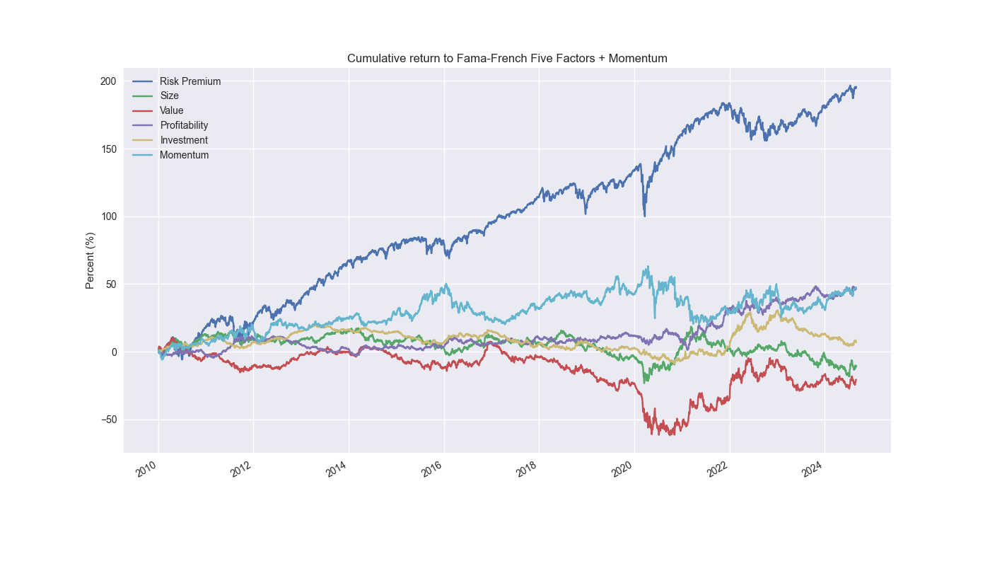
Whatever the case, while we can’t do justice to the logic behind the factors³, we can graph them to see if they tell us anything. We include the FF-Five plus Momentum in a cumulative return chart below.

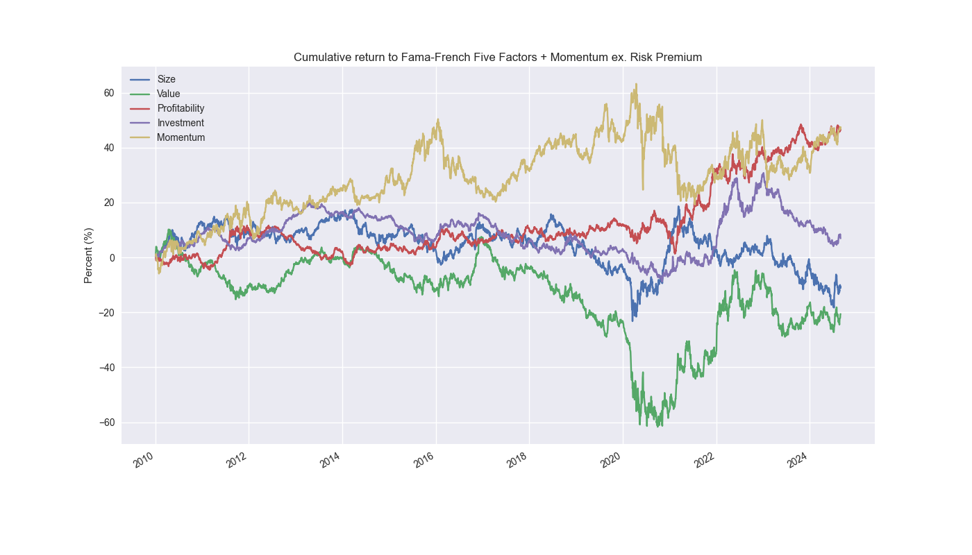
The Risk Premium seems to be the best factor. How do you invest in that? Buy and hold the market. Well, that doesn’t seem to a viable strategy if we want to charge lots of people money for our investing prowess. Let’s remove that one and see what we see.

Looks a bit like multi-colored spaghetti. But it does appear that Profitability and Momentum dominate the others. Maybe we can use profitability somehow. But, having been a sell-side analyst, forecasting profitability is arduous and prone to all sorts of errors – most of them unknown. Momentum, well that sounds kind of like science. So maybe we can use that to project more smarts than we actually have. Maybe if we throw in some other multi-syllabic math word like orthogonal or eigendecomposition we could add even further cache to our thumb in the wind prediction model.

Until we’ve got that narrative down, we’ll explore ways to quantify and forecast momentum since by the last chart it looks to be the most promising factor. We’ll focus on that tomorrow. Code below.

# Built using Python 3.10.19 and a virtual environment 

# Load libraries
import pandas as pd
import numpy as np
from datetime import datetime, timedelta
import matplotlib.pyplot as plt
from matplotlib.ticker import FuncFormatter
import pandas_datareader.data as pdr

plt.style.use('seaborn-v0_8')
plt.rcParams['figure.figsize'] = (14,8)

# Function to get FF-Factors
def get_fama_french_data(start_date, end_date):
    # Fetch Fama-French 5 Factors (Daily)
    ff_5_factors = pdr.get_data_famafrench('F-F_Research_Data_5_Factors_2x3_daily', start=start_date, end=end_date)[0]
    
    # Fetch Momentum Factor (Daily)
    momentum = pdr.get_data_famafrench('F-F_Momentum_Factor_daily', start=start_date, end=end_date)[0]
    
    # Combine the datasets
    factors = ff_5_factors.join(momentum)
    
    # Convert to percentage
    factors = factors / 100.0
    
    # Rename columns for clarity
    factors.columns = ['Mkt-RF', 'SMB', 'HML', 'RMW', 'CMA', 'RF', 'MOM']
    
    return factors

# Start and end dates
start_date = datetime(2000, 1, 1)
end_date = datetime(2024, 10, 1)

# Get FF-Factors
ff_factors = get_fama_french_data(start_date, end_date)
print(ff_factors.head())
print(ff_factors.tail())

# Graph factors
# All factors
((ff_factors.loc["2010-01-01":].drop(columns=["RF"]).cumsum())*100).plot()
plt.ylabel('Percent (%)')
plt.xlabel('')
plt.legend(['Risk Premium', 'Size', 'Value', 'Profitability','Investment', 'Momentum'])
plt.title('Cumulative return to Fama-French Five Factors + Momentum')
plt.savefig("images/ff-factors_cumul_return.png")
plt.show()

# Factors ex-Market Risk Premium
((ff_factors.loc["2010-01-01":].drop(columns=["Mkt-RF","RF"]).cumsum())*100).plot()
plt.ylabel('Percent (%)')
plt.xlabel('')
plt.legend(['Size', 'Value', 'Profitability','Investment', 'Momentum'])
plt.title('Cumulative return to Fama-French Five Factors + Momentum ex. Risk Premium')
plt.savefig("images/ff-factors_cumul_return_ex_mkt-rf.png")
plt.show()