Day 10: Residuals

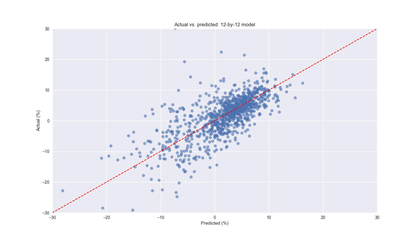
On Day 9 we conducted a walk-forward analysis on the 12-by-12 week lookback-look forward combination. We then presented the canonical the actual vs. predicted value graph with a \(45^o\) line overlay to show what a perfect forecast would look like. Here’s the graph again.

As noted previously, we limited the scale of the axes to make it easier to interpret. This omits some outliers, which we’ll touch on below. The main body of the graph shows a nice scattering of the data around the line. Since the data doesn’t appear to show more points above or below the line, it is probably not overly biased. Indeed, the frequency of predicted values above actual values is about 53%. The shape of the graph itself looks a bit a like a snowstorm – as opposed to shotgun blast – meaning the change in the error seems pretty consistent across the predictions. There is no evident non-linearity. On this account, the model seems pretty good from a statistics perspective.

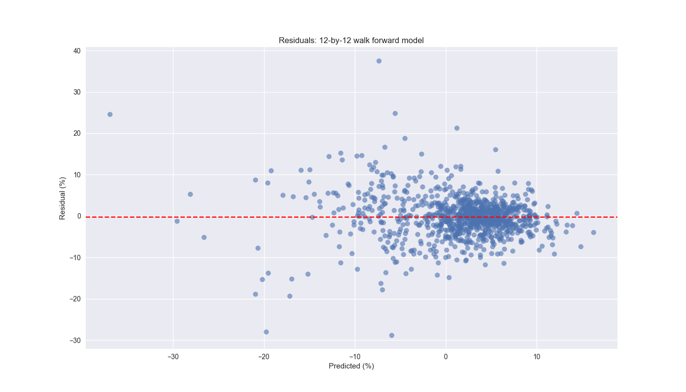
Nonetheless, we should still drill down into the error analysis to see if we can find evidence of non-constant variance.¹ This is mostly clearly shown when we graph the residual (actual less predicted value) against the predicted values below. True, the mean of the residuals (the dashed red line) is close to zero.² However, as the predictions drop below zero, the residuals increase. This extends for a bit and then jumps up to the massive outlier where the model predicts close to a 37% decline in the next 12-week return, but that return ends up only being a loss of 12%. Points for guessing. That was using data toward the end of the Global Financial Crisis.

These results suggest the model is not bad around the normal periods. But when the market is under extreme stress, watch out! We’ll also want to check for autocorrelation in the residuals – that is, the current value has some linear relationship with a prior or many prior values – but we’ll save that for the next post.

What are our initial takeaways? The model seems not overly biased or misspecified in the -10% to 10% region. But when you start to get outside that range, be careful! We’ll look at the errors in more detail tomorrow and then iterate different walk-forward combinations. Code below.

# Built using Python 3.10.19 and a virtual environment 

# Load libraries
import pandas as pd
import numpy as np
from datetime import datetime, timedelta
import statsmodels.api as sm
import matplotlib.pyplot as plt
from matplotlib.ticker import FuncFormatter

plt.style.use('seaborn-v0_8')
plt.rcParams['figure.figsize'] = (14,8)

# Load data and clean
df = yf.download('SPY', start='2000-01-01', end='2024-10-01')
df.columns = ['open', 'high', 'low', 'close', 'adj close', 'volume']
df.index.name = 'date'

# Create training set and downsample to weekly ending Friday
df_train = df.loc[:'2019-01-01', 'adj close'].copy()
df_w = pd.DataFrame(df_train.resample('W-FRI').last())
df_w.columns = ['price'] 
df_w.head()

# Create lookback/look forward model combinations
periods = [3, 6, 9, 12]
momo_dict = {}
for back in periods:
    for forward in periods:
        df_out = df_w.copy()
        df_out['ret_back'] = np.log(df_out['price']/df_out['price'].shift(back))
        df_out['ret_for'] = np.log(df_out['price'].shift(-forward)/df_out['price'])
        df_out = df_out.dropna()

        mod = sm.OLS(df_out['ret_for'], sm.add_constant(df_out['ret_back'])).fit()
        momo_dict[f"{back} - {forward}"] = {'data': df_out,
                                            'params': mod.params,
                                            'pvalues': mod.pvalues}

# Select model for testing and perform walk-forward analysis
test = momo_dict['12 - 12']['data']

train_pd = 13
test_pd = 1
tot_pd = train_pd + test_pd

fcst_dict = {}
for i in range(tot_pd, len(test), test_pd):
    train_df = test.iloc[i-tot_pd:i-test_pd, 1:]
    test_df = test.iloc[i-test_pd:i, 1:]
    
    # Ensure 'ret_back' is 2D by selecting it as a DataFrame, not a Series
    X_train = sm.add_constant(train_df[['ret_back']])
    if test_df.shape[0] > 1: 
        X_test = sm.add_constant(test_df[['ret_back']])
    else:
        X_test = sm.add_constant(test_df[['ret_back']], has_constant='add')

    # Fit the model
    mod_run = sm.OLS(train_df['ret_for'], X_train).fit()

    # Predict using the test data
    pred = mod_run.predict(X_test).values[0]

    # Calculate RMSE and average actual values
    rmse = np.sqrt(np.mean((pred - test_df['ret_for'].values) ** 2))
    actual = test_df['ret_for'].values[0]
    if test_df.shape[0] > 1:
        period = f"{str(test_df.index[0])[:10]} - {str(test_df.index[-1])[:10]}"
    else:
        period = f"{str(test_df.index[0])[:10]}"
    
    # Store forecast results
    fcst_dict[period] = {'rmse': rmse, 'actual': actual, 'predicted': pred}

# convert dictionary to dataframe
df_fcst = pd.DataFrame(fcst_dict).T

# Plot actual vs predicted
plt.figure()
plt.scatter(df_fcst['predicted']*100, df_fcst['actual']*100, alpha=0.6)
plt.plot([-30,30], [-30,30], 'r--', linewidth=1.5)
plt.xlim(-30,30)
plt.ylim(-30,30)
plt.xlabel("Predicted (%)")
plt.ylabel("Actual (%)")
plt.title('Actual vs. predicted: 12-by-12 model')
# plt.savefig("pred_act_3-3.png")
# plt.savefig("images/pred_act_12-12.png")
# plt.savefig("pred_act_3-3_all.png")
plt.show()

# Add residual
df_fcst['resid'] = df_fcst['actual'] - df_fcst['predicted']

# Print mean of residual
df_fcst['resid'].mean()

# Plot residual against predicted value
plt.figure()
plt.scatter(df_fcst['predicted']*100, df_fcst['resid']*100, alpha=0.6)
plt.axhline(df_fcst['resid'].mean()*100, color='red', linestyle='--')
plt.xlabel("Predicted (%)")
plt.ylabel("Residual (%)")
plt.title('Residuals: 12-by-12 walk forward model')
# plt.savefig("images/pred_act_12-12_resid.png")
plt.show()