Day 11: Autocorrelation

On Day 10, we analyzed the performance of the 12-by-12 model by examining the predicted values and residuals. Our initial takeaway suggested the model did seem not overly biased or misspecified in the -10% to 10% region. But when it gets outside that range, watch out! We suspected that there was some autocorrelation in the residuals, which we want to discuss today. There are different statistical tests for autocorrelation and normality that would take too long to explain in a blog post. However, graphing the correlation between current and lagged values (using a set number of lags) can help us see this visually. Throw in an area of significance and you’ve got a story even a sell-side analyst can understand!

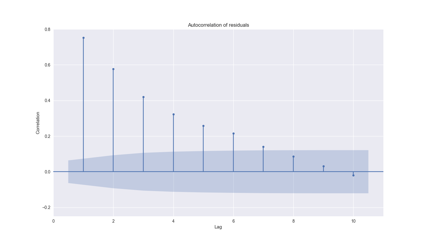
We graph the first 10 lags of the residuals below. The shaded area is the confidence interval indicating whether the result is statistically significant – that is, if it falls out of the shade area, then it’s significant!

We see that lags 1-7 hit the nail on the head. This suggests the present model hasn’t identified critical time dependencies or is just incorrect. Sad face. There are a bunch of ways to figure out which one it might be and fix it, but that would take us down a rabbit hole of stats modeling.¹ At this stage we’re not really trying to improve the 12-by-12 model. In fact, we’re only trying to see if we can find a way to approximate the real time implementation of a momentum model to generate a relatively accurate forecast to use as a signal for a trading strategy.

Common sense suggests we shouldn’t expect a straightforward model like what we’ve put forth thus far to be all that predictive. If it were, then investing would be as easy as pulling a Jupyter notebook from Kaggle, sending the signals to your favorite broker who favors Lincoln green, and then counting the Benjamins all the while playing first person shooter games as a fat one…let’s move on.

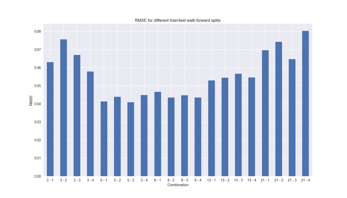
Recall, our walk-forward analysis started with a rolling 13-step window to train a model with a single step forecast (or test). How do we know if that 13-by-1 combination provides the best results? Why not 17-by-5? We don’t know, so why not iterate? Now we finally get to use Fibonacci sequences! We use the Fibonacci numbers from 3 to 21 as the training steps and 1 through 4 forward steps for the forecasts, yielding 20 different scenarios.² We then use the root mean-squared error (RMSE) as the way to judge performance. Here’s the graph of the output.

As shown above, RMSE tends to decline when you increase the training period to a valley encompassing the 5-by-1 to the 13-by-4 combination. It is unclear why the jump from 13 to 21 periods sees an increase in RMSE. While the difference might be small – ~3% points – that can be the critical threshold between under and outperformance, especially when compounding over multiple periods. We’ll discuss RMSE and more tomorrow. Code below.

# Built using Python 3.10.19 and a virtual environment 

# Load libraries
import pandas as pd
import numpy as np
from datetime import datetime, timedelta
import statsmodels.api as sm
import matplotlib.pyplot as plt
from matplotlib.ticker import FuncFormatter
from statsmodels.graphics.tsaplots import plot_acf
from statsmodels.tsa.stattools import acf

plt.style.use('seaborn-v0_8')
plt.rcParams['figure.figsize'] = (14,8)

# Load data and clean
df = yf.download('SPY', start='2000-01-01', end='2024-10-01')
df.columns = ['open', 'high', 'low', 'close', 'adj close', 'volume']
df.index.name = 'date'

# Create training set and downsample to weekly ending Friday
df_train = df.loc[:'2019-01-01', 'adj close'].copy()
df_w = pd.DataFrame(df_train.resample('W-FRI').last())
df_w.columns = ['price'] 
df_w.head()

# Create lookback/look forward model combinations
periods = [3, 6, 9, 12]
momo_dict = {}
for back in periods:
    for forward in periods:
        df_out = df_w.copy()
        df_out['ret_back'] = np.log(df_out['price']/df_out['price'].shift(back))
        df_out['ret_for'] = np.log(df_out['price'].shift(-forward)/df_out['price'])
        df_out = df_out.dropna()

        mod = sm.OLS(df_out['ret_for'], sm.add_constant(df_out['ret_back'])).fit()
        momo_dict[f"{back} - {forward}"] = {'data': df_out,
                                            'params': mod.params,
                                            'pvalues': mod.pvalues}

# Select model for testing and perform walk-forward analysis
test = momo_dict['12 - 12']['data']

train_pd = 13
test_pd = 1
tot_pd = train_pd + test_pd

fcst_dict = {}
for i in range(tot_pd, len(test), test_pd):
    train_df = test.iloc[i-tot_pd:i-test_pd, 1:]
    test_df = test.iloc[i-test_pd:i, 1:]
    
    # Ensure 'ret_back' is 2D by selecting it as a DataFrame, not a Series
    X_train = sm.add_constant(train_df[['ret_back']])
    if test_df.shape[0] > 1: 
        X_test = sm.add_constant(test_df[['ret_back']])
    else:
        X_test = sm.add_constant(test_df[['ret_back']], has_constant='add')

    # Fit the model
    mod_run = sm.OLS(train_df['ret_for'], X_train).fit()

    # Predict using the test data
    pred = mod_run.predict(X_test).values[0]

    # Calculate RMSE and average actual values
    rmse = np.sqrt(np.mean((pred - test_df['ret_for'].values) ** 2))
    actual = test_df['ret_for'].values[0]
    if test_df.shape[0] > 1:
        period = f"{str(test_df.index[0])[:10]} - {str(test_df.index[-1])[:10]}"
    else:
        period = f"{str(test_df.index[0])[:10]}"
    
    # Store forecast results
    fcst_dict[period] = {'rmse': rmse, 'actual': actual, 'predicted': pred}

# convert dictionary to dataframe
df_fcst = pd.DataFrame(fcst_dict).T

# Add residual
df_fcst['resid'] = df_fcst['actual'] - df_fcst['predicted']
df_fcst['resid'].mean()

# Find autocorrelation values
acf_values = acf(df_fcst['resid'].dropna())
acf_values[0] = np.nan

# Plot ACF
plot_acf(df_fcst['resid'].dropna(), zero=False, lags=10)
plt.ylim(-0.25, .80)
plt.ylabel('Correlation')
plt.xlabel('Lag')
plt.title('Autocorrelation of residuals')
plt.savefig('images/resid_autocor.png')
plt.show()

# Set iteration and run combinations of train/forecast steps
train_pds = [3, 5, 8, 13, 21]
test_pds = [1, 2, 3, 4]

df_pd = pd.DataFrame(columns = ['combo','rmse', 'rmse_scaled'])
count = 0
for i in train_pds:
    for j in test_pds:
        tot_pd = i + j 
        actual = []
        predicted = []
        for k in range(tot_pd, len(test), j):
            train_df = test.iloc[k-tot_pd:k-j, 1:]
            test_df = test.iloc[k-j:k, 1:]
            
            # Ensure 'ret_back' is 2D by selecting it as a DataFrame, not a Series
            X_train = sm.add_constant(train_df[['ret_back']])
            if test_df.shape[0] > 1: 
                X_test = sm.add_constant(test_df[['ret_back']])
            else:
                X_test = sm.add_constant(test_df[['ret_back']], has_constant='add')

            # Fit the model
            mod_run = sm.OLS(train_df['ret_for'], X_train).fit()

            # Predict using the test data
            mod_pred = mod_run.predict(X_test).values[0]
            test_act = test_df['ret_for'].values[0]
            if j < 1:
                predicted.append(mod_pred)
                actual.append(test_act)
            else:
                predicted.append(np.array(mod_pred).mean())
                actual.append(np.array(test_act).mean())

        pred = np.array(predicted)
        act = np.array(actual)
        rmse = np.sqrt(np.mean((act - pred)**2))
        rmse_scaled = rmse/act.mean()
        df_pd.loc[count] = [f"{i} - {j}", rmse, rmse_scaled]
        count += 1

# Plot RMSE
df_pd.set_index('combo')['rmse'].plot(kind='bar', rot=0)
plt.xlabel("Combination")
plt.ylabel("RMSE")
plt.title('RMSE for different train/test walk forward splits')
plt.show()