Day 13: Backtest I

Unlucky 13! Or contrarian indicator? There’s really nothing so heartwarming as magical thinking. Whatever the case, on Day 12 we iterated through the 320 different model and train step iterations to settle on 10 potential candidates. Today, we look at the best performing candidate and discuss the process to see if the forecasts produce a viable trading strategy.

As we noted before, we could have launched directly into testing Fibonacci retracements with Bollinger Band breakouts filtered by Chaikin Volatility, but what would be the thesis as to why these indicators work better than others? Instead, we built 16 predictive models for momentum, iterated through different train/forecast combinations, performing walk-forward analyses to identify some potential candidates. While we wouldn’t say any of the models we have are all that magnificent, we have an evidenced-based thesis to go on.

The next step is to turn these predictions into trading signals. There are lots of ways to do this, but the simplest is to say if the prediction in the next period is positive, go long, if not do nothing. We can also add in a short version if the prediction is negative. But we’ll group those into separate tests – namely, long-only, and long-short. Of course, we can get fancier. If the prediction is greater than the 5-step moving average, or above a 1.5 standard deviation move, or equal to the solar flare index scaled by the square of time since the prior peak, then go long. The point at this stage is not so much to get the correct trading signal, but to analyze how predictions translate into trading signals. A good prediction may not yield a good trading signal and vice versa.

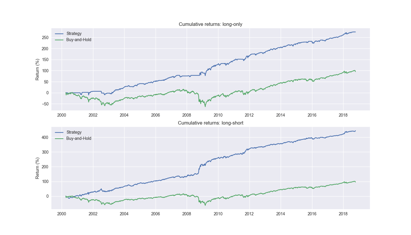
How this works is the following. We use the 12-by-12/5-by-1 combination we mentioned yesterday. Recall that is the 12-week lookback/12-week look forward set. We train a model on blocks of five instances of the 12-week lookbacks to build a model to forecast the next 12-week momentum as the target variable. We then step forward using the 5-step model we just built to forecast the 12-week momentum based on the next step in the 12-week lookback series. We then aggregate all those forecasts and if the model predicts a positive return in the next 12 weeks, we go long at the close of the current week and hold until it predicts a negative return for the long-only strategy or close the position and short for the long-short strategy. Let’s look at the performance.

Wow! That is about all we can say. Both long-only and long-short absolutely knock the cover off the ball. Given this, we’re going to end our blog here and immediately start trading this strategy. Have a nice year!

Wait a minute. Shouldn’t we be particularly skeptical of this performance? Does it seem realistic that such a relatively simple model with a few modifications could achieve such stellar results when there are legions of CFAs¹, MBAs, and PhDs trying to beat the market? We’ll answer that question in tomorrow’s post. Spoiler alert: we intentionally introduced a critical error in our data aggregation that will become patently clear. Stay tuned!

Code below.

# Built using Python 3.10.19 and a virtual environment 

# Load libraries
import pandas as pd
import numpy as np
from datetime import datetime, timedelta
import statsmodels.api as sm
import matplotlib.pyplot as plt
import yfinance as yf

plt.style.use('seaborn-v0_8')
plt.rcParams['figure.figsize'] = (14,8)

# Function to get data
def get_spy_weekly_data() -> pd.DataFrame:
    df = yf.download('SPY', start='2000-01-01', end='2024-10-01')
    df.columns = ['open', 'high', 'low', 'close', 'adj close', 'volume']
    df.index.name = 'date'

    # Create training set and downsample to weekly ending Friday
    df_train = df.loc[:'2019-01-01', 'adj close'].copy()
    df_w = pd.DataFrame(df_train.resample('W-FRI').last())
    df_w.columns = ['price'] 

    return df_w

# Get data
df_w = get_spy_weekly_data()

# Create momentum dictionary
periods = [3, 6, 9, 12]
momo_dict = {}
for back in periods:
    for forward in periods:
        df_out = df_w.copy()
        df_out['ret_back'] = np.log(df_out['price']/df_out['price'].shift(back))
        df_out['ret_for'] = np.log(df_out['price'].shift(-forward)/df_out['price'])
        df_out = df_out.dropna()

        mod = sm.OLS(df_out['ret_for'], sm.add_constant(df_out['ret_back'])).fit()
        momo_dict[f"{back} - {forward}"] = {'data': df_out,
                                            'params': mod.params,
                                            'pvalues': mod.pvalues}

# Prepare model
model_name = '12 - 12'
mod_look_forward = 12
train_pd = 5
test_pd = 1
tot_pd = train_pd + test_pd

# Create trading dataframe
df_trade = momo_dict[model_name]['data'].copy()

# Run model with train/forecast steps
trade_pred = []
for i in range(tot_pd, len(df_trade)+1, test_pd):
    train_df = df_trade.iloc[i-tot_pd:i-test_pd, 1:]
    test_df = df_trade.iloc[i-test_pd:i, 1:]

    # Ensure 'ret_back' is 2D by selecting it as a DataFrame, not a Series
    X_train = sm.add_constant(train_df[['ret_back']])
    if test_df.shape[0] > 1:
        X_test = sm.add_constant(test_df[['ret_back']])
    else:
        X_test = sm.add_constant(test_df[['ret_back']], has_constant='add')

    # Fit the model
    mod_run = sm.OLS(train_df['ret_for'], X_train).fit()

    # Predict using the test data
    mod_pred = mod_run.predict(X_test).values
    trade_pred.extend(mod_pred)

# Add predictions to dataframe
df_trade['pred'] = np.concatenate((np.repeat(np.nan,train_pd), np.array(trade_pred)))

# Generate returns
df_trade['ret'] = np.log(df_trade['price']/df_trade['price'].shift(1))

# Generate signals
df_trade['signal'] = np.where(df_trade['pred'] == np.nan, np.nan, np.where(df_trade['pred'] > 0, 1, 0))
df_trade['signal_sh'] = np.where(df_trade['pred'] == np.nan, np.nan, np.where(df_trade['pred'] >= 0, 1, -1))

# Generate strategy returns
df_trade['strat_ret'] = df_trade['signal'].shift(1) * df_trade['ret']
df_trade['strat_ret_sh'] = df_trade['signal_sh'].shift(1) * df_trade['ret']

# Plot cumulative performance plot for long-only and long-shor
fig, (ax1, ax2) = plt.subplots(2,1)

top = df_trade[['strat_ret_snoop', 'ret']].cumsum()
bottom = df_trade[['strat_ret_snoop_sh', 'ret']].cumsum()

ax1.plot(top.index, top.values*100)
ax1.set_xlabel("")
ax1.set_ylabel("Return (%)")
ax1.legend(['Strategy', 'Buy-and-Hold'], loc="upper left")
ax1.set_title("Cumulative returns: long-only")

ax2.plot(bottom.index, bottom.values*100)
ax2.set_xlabel("")
ax2.set_ylabel("Return (%)")
ax2.legend(['Strategy', 'Buy-and-Hold'], loc="upper left")
ax2.set_title("Cumulative returns: long-short")

plt.show()