Day 17: Drawdowns

On Day 16, we showed the adjusted 12-by-12 strategy with full performance metrics against buy-and-hold, the 60-40 SPY-IEF ETF portfolio, and the 200-day SMA strategy. In all cases, it tended to perform better than the benchmarks. However, against the 200-day SMA that performance came primarily at the end of the period. This begs the question of what to make of the performance differences between the 12-by-12 and 200-day SMA strategies.

The 12-by-12 strategy derived most of its outperformance from the last three years of the backtest. For a good portion, it actually underperformed the 200-day SMA. Additionally, the difference in risk-adjusted returns between the two strategies, as judged by the Sharpe Ratio, was de minimis. On this account, we’ll need to drill down into drawdowns to see if that favors one strategy over the over.

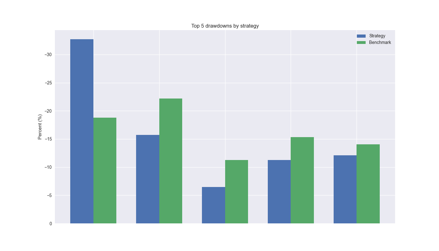
When we look at the magnitude of top 5 drawdowns, we see that the 12-by-12 strategy certainly exceeds the 200-day SMA by almost 14% points. However, for the remaining periods it is below the 200-day. The average difference of maximum drawdowns in the top 5 periods is a less than 1% point.

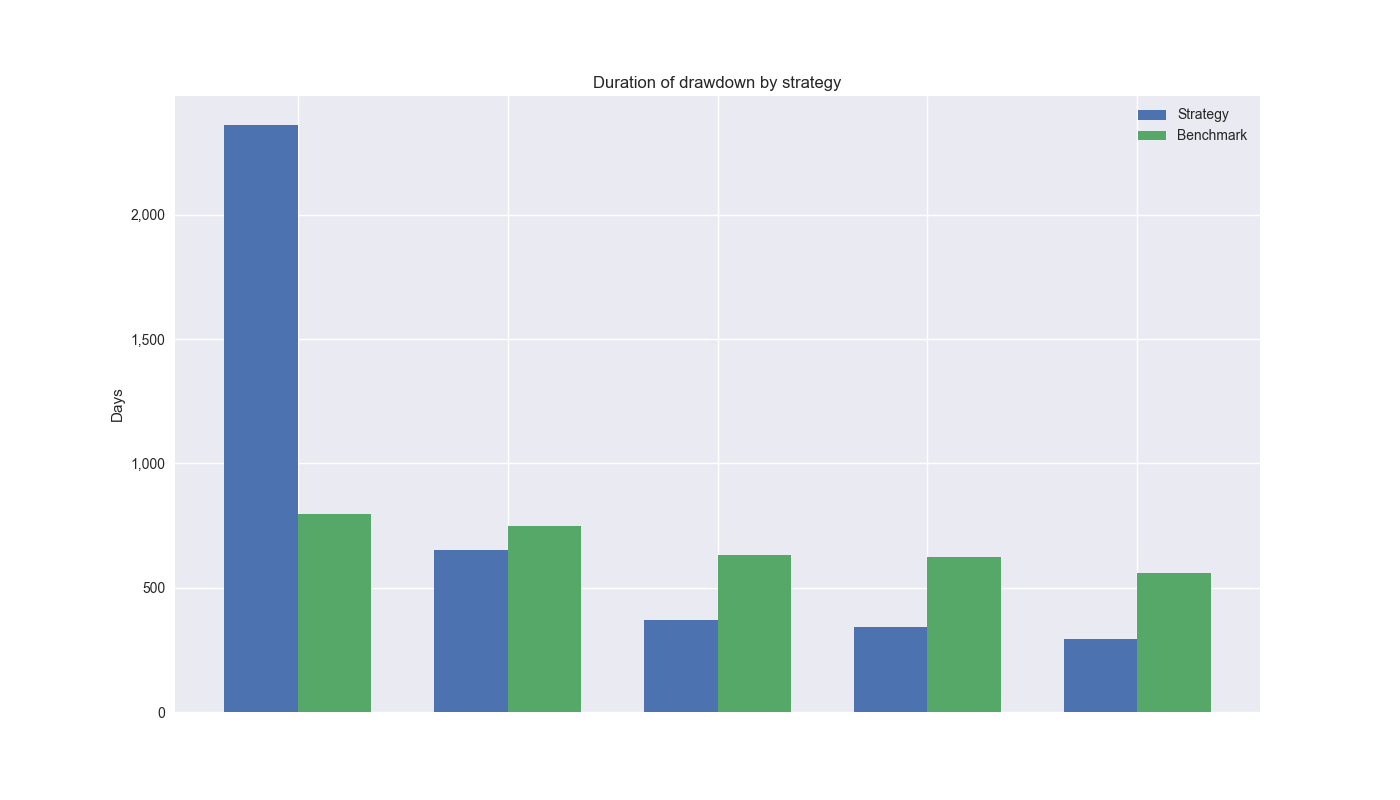
Next let’s look at drawdown duration. Again, the 12-by-12 massively exceeds the 200-day for the top spot. But the 200-day beats the 12-by-12 for the remainder. In this case, the 12-by-12 is decidedly worse off, as the average difference in drawdown periods is about 132 days greater than the 200-day.

Let’s take stock. While the 12-by-12 modestly outperforms on a cumulative performance basis, it’s risk-adjusted return is not significantly different from the 200-day¹. The 12-by-12 has a single drawdown that exceeds the 200-day, but the differences are not meaningful on average. Finally, the 12-by-12 does suffer a single drawdown period that far exceeds the 200-day individually and over the average. Should we favor the 12-by-12 or stick with Hello World – the 200-day?

Before we answer that question, it is important to note that the main periods of underperformance and outperformance for the 12-by-12 come at the beginning and end of the analysis timeframe. Notably, the aftermath of the Tech bubble (e.g., underperformance) and the halcyon years prior to Covid-19. Recall, we stopped our analysis prior to 2019 to have around five years of data once we’d found a strategy that seemed attractive to test out-of-sample. So should we weight this barbell performance equally with the intermediate period that includes the Global Financial Crisis?

The barbell results certainly speak to regime switching and may reveal how one strategy performs better in different regimes. The decision to employ one or the other could now turn on risk preferences and explainability, as opposed to performance results. No one wants to endure over 1,000 days of underperformance. But who is to say there will be another Tech Bubble or pre-Covid period? What if we just looked at the 2005-2015 period? Guess what 12-by-12 outperforms by 30% points! But isn’t that cherry-picking too?

While these questions are relevant, they’re hard to answer without a crystal ball. That said, we can return to the recommendations of Marcos Lopéz de Prado and simulate future returns. We’ll look at that in detail in our next post. Code below.

# Built using Python 3.10.19 and a virtual environment 
# Load libraries
import pandas as pd
import numpy as np
from datetime import datetime, timedelta
import statsmodels.api as sm
import matplotlib.pyplot as plt
import yfinance as yf
from matplotlib.ticker import FuncFormatter

plt.style.use('seaborn-v0_8')
plt.rcParams['figure.figsize'] = (14,8)

# Function to get data
def get_spy_weekly_data() -> pd.DataFrame:
    df = yf.download('SPY', start='2000-01-01', end='2024-10-01')
    df.columns = ['open', 'high', 'low', 'close', 'adj close', 'volume']
    df.index.name = 'date'

    # Create training set and downsample to weekly ending Friday
    df_train = df.loc[:'2019-01-01', 'adj close'].copy()
    df_w = pd.DataFrame(df_train.resample('W-FRI').last())
    df_w.columns = ['price'] 

    return df_w

# Get data
df_w = get_spy_weekly_data()

# Create momentum dictionary
periods = [3, 6, 9, 12]
momo_dict = {}
for back in periods:
    for forward in periods:
        df_out = df_w.copy()
        df_out['ret_back'] = np.log(df_out['price']/df_out['price'].shift(back))
        df_out['ret_for'] = np.log(df_out['price'].shift(-forward)/df_out['price'])
        df_out = df_out.dropna()

        mod = sm.OLS(df_out['ret_for'], sm.add_constant(df_out['ret_back'])).fit()
        momo_dict[f"{back} - {forward}"] = {'data': df_out,
                                            'params': mod.params,
                                            'pvalues': mod.pvalues}

# Prepare model
model_name = '12 - 12'
mod_look_forward = 12
train_pd = 5
test_pd = 1
tot_pd = train_pd + test_pd

# Create trading dataframe
df_trade = momo_dict[model_name]['data'].copy()

# Run model with train/forecast steps
trade_pred = []
for i in range(tot_pd, len(df_trade)+1, test_pd):
    train_df = df_trade.iloc[i-tot_pd:i-test_pd, 1:]
    test_df = df_trade.iloc[i-test_pd+mod_look_forward-1:i-test_pd+mod_look_forward, 1:]

    # Ensure 'ret_back' is 2D by selecting it as a DataFrame, not a Series
    X_train = sm.add_constant(train_df[['ret_back']])
    if test_df.shape[0] > 1:
        X_test = sm.add_constant(test_df[['ret_back']])
    else:
        X_test = sm.add_constant(test_df[['ret_back']], has_constant='add')

    # Fit the model
    mod_run = sm.OLS(train_df['ret_for'], X_train).fit()

    # Predict using the test data
    mod_pred = mod_run.predict(X_test).values
    trade_pred.extend(mod_pred)

# Test for lenghth
assert len(trade_pred) + mod_look_forward + train_pd - 1 == len(df_trade) 

# Add predictions to dataframe
df_trade['pred'] = np.concatenate((np.repeat(np.nan, mod_look_forward + train_pd - 1), np.array(trade_pred)))

# Generate returns
df_trade['ret'] = np.log(df_trade['price']/df_trade['price'].shift(1))

# Generate signals
df_trade['signal'] = np.where(df_trade['pred'] == np.nan, np.nan, np.where(df_trade['pred'] > 0, 1, 0))
df_trade['signal_sh'] = np.where(df_trade['pred'] == np.nan, np.nan, np.where(df_trade['pred'] >= 0, 1, -1))

# Generate strategy returns
df_trade['strat_ret'] = df_trade['signal'].shift(1) * df_trade['ret']
df_trade['strat_ret_sh'] = df_trade['signal_sh'].shift(1) * df_trade['ret']

# Create 200-day strategy
df_200 = df_w.copy()
df_200.columns = ['price']
df_200 = df_200.resample('W-FRI').last()
# 40 weeks = 200 days
df_200['sma_200'] = df_200['price'].rolling(40).mean()
df_200['ret'] = np.log(df_200['price']/df_200['price'].shift(1))
df_200['signal'] = np.where(df_200['price'] > df_200['sma_200'], 1, 0)
df_200['strat_ret'] = df_200['signal'].shift(1)*df_200['ret']
df_200_bench = df_200.loc[df_trade['strat_ret'].index[0]:df_trade['strat_ret'].index[-1]]

# Function from tearsheet for drawdowns
def get_drawdown_periods(cumulative_returns):
    peak = cumulative_returns.cummax()
    drawdown = cumulative_returns - peak

    end_of_dd = drawdown[drawdown == 0].index
    dd_periods = []
    start = cumulative_returns.index[0]
    for end in end_of_dd:
        if start < end:
            period = (start, end)
            dd_periods.append(period)
        start = end

    return drawdown, dd_periods
# Get drawdowns and periods
dd_12_12, pd_12_12 = get_drawdown_periods(df_trade['strat_ret'].cumsum())
dd_200, pd_200 = get_drawdown_periods(df_200_bench['strat_ret'].cumsum())

# Sort drawdown perios 
top_dd_pds_12 = sorted(pd_12_12, key=lambda x: (x[1] - x[0]).days, reverse=True)[:5]
top_dd_pds_200 = sorted(pd_200, key=lambda x: (x[1] - x[0]).days, reverse=True)[:5]
top_5_12 = [(end - start).days for start, end in top_dd_pds_12]
top_5_200 = [(end - start).days for start, end in top_dd_pds_200]

# Get drawdown magnitude
peak_12 = df_trade['strat_ret'].cumsum().cummax()
drawdown_12 = df_trade['strat_ret'].cumsum() - peak_12

peak_200 = df_200_bench['strat_ret'].cumsum().cummax()
drawdown_200 = df_200_bench['strat_ret'].cumsum() - peak_200

drawdown_12[drawdown_12 != 0.0].drop_duplicates().nsmallest(5)
drawdown_200[drawdown_200 != 0.0].drop_duplicates().nsmallest(5)

top_five_12_min = [drawdown_12[start:end].min()*100 for start, end in top_dd_pds_12]
top_five_200_min = [drawdown_200[start:end].min()*100 for start, end in top_dd_pds_200]

# Plot top 5 drawdowns by magnitude
x = np.arange(len(top_five_12_min))
width = 0.35  # Width of the bars

fig, ax = plt.subplots()

# Plotting bars side by side
bar1 = ax.bar(x - width/2, top_five_12_min, width, label='Strategy')
bar2 = ax.bar(x + width/2, top_five_200_min, width, label='Benchmark')

# Adding labels, title, and legend
ax.set_xlabel('')
ax.set_ylabel('Percent (%)')
ax.set_title('Top 5 drawdowns by strategy')
ax.set_xticks(x)
ax.set_xticklabels("")
ax.legend()
ax.invert_yaxis()
plt.show()

# Plot top 5 drawdown period comparisons
x = np.arange(len(top_5_12))
width = 0.35  # Width of the bars

fig, ax = plt.subplots()

# Plotting bars side by side
bar1 = ax.bar(x - width/2, top_5_12, width, label='Strategy')
bar2 = ax.bar(x + width/2, top_5_200, width, label='Benchmark')

# Adding labels, title, and legend
ax.set_xlabel('')
ax.set_ylabel('Days')
ax.set_title('Duration of drawdown by strategy')
ax.set_xticks(x)
ax.set_xticklabels("")
ax.legend()
ax.yaxis.set_major_formatter(FuncFormatter(lambda x, p: f'{int(x):,}'))
plt.show()