Day 19: Circular Sample

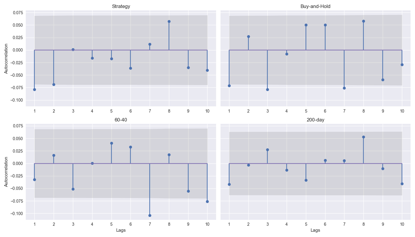
On Day 18 we started to discuss simulating returns to quantify the probability of success for a strategy out-of-sample. The reason for this was we were unsure whether or how much to merit the 12-by-12’s performance relative to the 200-Day SMA. We discussed various simulation techniques, but we settled on historical sampling that accounts for autocorrelation of returns. We then showed the autocorrelation plots for the strategy and the three benchmarks – buy-and-hold, 60-40, and 200-day – with up to 10 lags. Let’s show that again and discuss.

As shown on the graph above, the correlation coefficients are relatively modest, ranging between -10% and 10%. The significance of these coefficients is also small. The 12-by-12 strategy has two significant lags (1 and 2), buy-and-hold has three (1, 3, and 7), the 60-40 has one (7), and the 200-day (surprisingly!) has none. We suspect these results are partly explained by the duration used – namely, weekly – but won’t delve into that.

Given these results, which block should we use? This is where the fine art of backtesting comes into play. There is no deterministic way to answer this. However, our intuition suggests using buy-and-hold as the guide and the 3 and 7-week lag as the blocks is the way to go. The reason: the strategy will follow the patterns of the underlying so we should do our best to simulate the underlying distribution. Let’s dive in.

As this will actually involve several iterations within the code, we’ll first look at the 200-day SMA vs. buy-and-hold to ground the analysis. After that, we’ll run another iteration with the 12-by-12 strategy. For those interested in the steps of how we do this feel free to look below our code where we outline the algorithm. Let’s move to results.

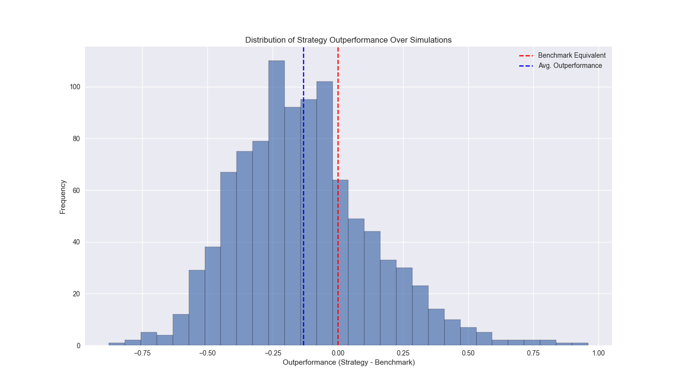
Our plan is forecast the likelihood a strategy will outperform buy-and-hold over a five year period. We sample three return blocks with replacement and append them together to create a five-year long time series. We repeat 1,000 times. We plot a histogram of the outperformance of the cumulative returns to the strategy vs. buy-and-hold. As one can see, at 13% points of underperformance (the blue dashed line), the 200-day’s mean is below the benchmark equivalent cut-off, where the strategy and benchmark achieve similar results, as shown by the red dashed line.

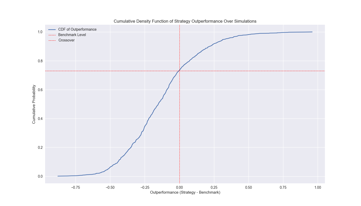
We also graph the empirical cumulative distribution function plot if that is more to the reader’s taste. The point where the two red lines cross is where the strategy begins to outperform buy-and-hold.

The crossover point is just below 27%. Hence, we can say that the frequency in which the 200-day outperforms buy-and-hold is about a quarter of the time. That doesn’t mean that in the future there’s precisely only a 25% chance the 200-day will outperform. Just that we shouldn’t assume we even have a 50/50 chance to outperform based on historical simulations. The Sharpe ratio fares better, however, with the strategy beating buy-and-hold over 30% of the time. Tomorrow we’ll run the circular block algorithm on the 12-by-12 strategy. Stay tuned.

Code below.

# Built using Python 3.10.19 and a virtual environment 


# Load libraries
import pandas as pd
import numpy as np
import yfinance as yf
from datetime import datetime, timedelta
import statsmodels.api as sm
import matplotlib.pyplot as plt
from matplotlib.ticker import FuncFormatter
from utils_intraday import *
from statsmodels.graphics.tsaplots import plot_acf
from statsmodels.tsa.stattools import acf
from tqdm import tqdm

plt.style.use('seaborn-v0_8')
plt.rcParams['figure.figsize'] = (14,8)

def get_spy_weekly_data() -> pd.DataFrame:
    df = yf.download('SPY', start='2000-01-01', end='2024-10-01')
    df.columns = ['open', 'high', 'low', 'close', 'adj close', 'volume']
    df.index.name = 'date'

    # Create training set and downsample to weekly ending Friday
    df_train = df.loc[:'2019-01-01', 'adj close'].copy()
    df_w = pd.DataFrame(df_train.resample('W-FRI').last())
    df_w.columns = ['price'] 

    return df_w

df_w = get_spy_weekly_data()

# Create momentum dictionary
periods = [3, 6, 9, 12]
momo_dict = {}
for back in periods:
    for forward in periods:
        df_out = df_w.copy()
        df_out['ret_back'] = np.log(df_out['price']/df_out['price'].shift(back))
        df_out['ret_for'] = np.log(df_out['price'].shift(-forward)/df_out['price'])
        df_out = df_out.dropna()

        mod = sm.OLS(df_out['ret_for'], sm.add_constant(df_out['ret_back'])).fit()
        momo_dict[f"{back} - {forward}"] = {'data': df_out,
                                            'params': mod.params,
                                            'pvalues': mod.pvalues}

# Prepare model
model_name = '12 - 12'
mod_look_forward = 12
train_pd = 5
test_pd = 1
tot_pd = train_pd + test_pd

df_trade = momo_dict[model_name]['data'].copy()

trade_pred = []
for i in range(tot_pd, len(df_trade)+1, test_pd):
    train_df = df_trade.iloc[i-tot_pd:i-test_pd, 1:]
    test_df = df_trade.iloc[i-test_pd+mod_look_forward-1:i-test_pd+mod_look_forward, 1:]

    # Ensure 'ret_back' is 2D by selecting it as a DataFrame, not a Series
    X_train = sm.add_constant(train_df[['ret_back']])
    if test_df.shape[0] > 1:
        X_test = sm.add_constant(test_df[['ret_back']])
    else:
        X_test = sm.add_constant(test_df[['ret_back']], has_constant='add')

    # Fit the model
    mod_run = sm.OLS(train_df['ret_for'], X_train).fit()

    # Predict using the test data
    mod_pred = mod_run.predict(X_test).values
    trade_pred.extend(mod_pred)

df_trade['pred'] = np.concatenate((np.zeros(mod_look_forward + train_pd - 1), np.array(trade_pred)))
df_trade['ret'] = np.log(df_trade['price']/df_trade['price'].shift(1))

df_trade['signal'] = np.where(df_trade['pred'] > 0, 1, 0)
df_trade['signal_sh'] = np.where(df_trade['pred'] >= 0, 1, -1)

df_trade['strat_ret'] = df_trade['signal'].shift(1) * df_trade['ret']
df_trade['strat_ret_sh'] = df_trade['signal_sh'].shift(1) * df_trade['ret']

# Load data for 60-40
df = pd.read_csv('data/spy_ief_close.csv', parse_dates=['date'], index_col='date')
df_bw =  pd.DataFrame(df.resample('W-FRI').last())
df_bw[['ief_chg', 'spy_chg']] = df_bw[['ief','spy']].apply(lambda x: np.log(x/x.shift(1)))

end_date_bench = df_trade.index[-1].strftime("%Y-%m-%d")
bench_returns = df_bw[['ief_chg', 'spy_chg']].copy()
bench_returns = bench_returns.loc[:end_date_bench]
bench_returns = bench_returns.dropna()

strat_returns_start = bench_returns.index[0].strftime("%Y-%m-%d")
strat_returns = df_trade['strat_ret'].copy()
strat_returns = strat_returns.loc[strat_returns_start:]

# Create 60-40 benchmark
# See Day 18 for calculate_portfolio_performance() function
weights = [0.4,0.6]
bench_60_40_rebal = calculate_portfolio_performance(weights, bench_returns, rebalance=False, frequency='quarter')
bench_60_40_rebal.index = bench_60_40_rebal.index.tz_localize(None) #type:ignore

# Create 200-day benchmark
df_200 = df_w.copy()
df_200.columns = ['price']
df_200 = df_200.resample('W-FRI').last()
# 40 weeks = 200 days
df_200['sma_200'] = df_200['price'].rolling(40).mean()
df_200['ret'] = np.log(df_200['price']/df_200['price'].shift(1))
df_200['signal'] = np.where(df_200['price'] > df_200['sma_200'], 1, 0)
df_200['strat_ret'] = df_200['signal'].shift(1)*df_200['ret']
df_200_bench = df_200.loc[df_trade['strat_ret'].index[0]:df_trade['strat_ret'].index[-1]]

# Plot ACF
return_data = [strat_returns, bench_returns['spy_chg'], bench_60_40_rebal, df_200_bench['strat_ret']]
names = ['Strategy', 'Buy-and-Hold', '60-40', '200-day']

fig, axs = plt.subplots(2, 2, sharey=True)

for idx, (data, name) in enumerate(zip(return_data, names)):
    # Calculate the autocorrelation
    acf_values, confint = acf(data.dropna(), nlags=10, alpha=0.05) #type: ignore

    lower_bound = confint[1:, 0] - acf_values[1:]
    upper_bound = confint[1:, 1] - acf_values[1:]

    # Find the correct subplot (axs[0, 0], axs[0, 1], etc.)
    ax = axs[idx // 2, idx % 2]
    ax.stem(range(1, len(acf_values)), acf_values[1:])
    
    # Set x-ticks to match lag numbers
    ax.set_xticks(range(1, len(acf_values)))
    ax.set_xticklabels(range(1, len(acf_values)))

    # Add shaded area for confidence interval
    ax.fill_between(range(1, len(acf_values)), upper_bound, lower_bound, color='gray', alpha=0.2)
    
    ax.set_title(name)
    if idx > 1:
        ax.set_xlabel("Lags")
    if idx % 2 == 0:
        ax.set_ylabel("Autocorrelation")

plt.tight_layout()
plt.show()


# Circular block
data = df_w.apply(lambda x: np.log(x/x.shift(1))).dropna().copy()
data = data.loc[:'2019-01-01']
block_size = 3
data_idx = len(data) - 1
# data_len = len(data)
data_len = int(52*5)
iter = data_len // block_size 
adder = data_len % block_size
block_data = []

# Create simulated returns
np.random.seed(42)
for _ in tqdm(range(1000), desc='Simulation'):
    dat = []
    for _ in range(iter):
        start = np.random.choice(data_idx, 1)[0]
        end = start+block_size
        out = data.iloc[start:end]
        if end > data_idx + 1:
            new_end = end - data_idx - 1
            new_out = data.iloc[:new_end]
            out = pd.concat([out, new_out])
        dat.extend(out.values)
    if adder:
        new_start = np.random.choice(data_idx, 1)[0]
        new_end = new_start+adder
        out_add = data.iloc[new_start:new_end]
        if new_end > data_idx + 1:
            s_end = new_end - data_idx - 1
            s_end = s_end if s_end < adder else adder - 1 
            new_out = data.iloc[:s_end]
            out_add = pd.concat([out_add, new_out])
        dat.extend(out_add.values)
    block_data.append(dat)

# create trading strategy for each simulation
lst_sim = []
for dt in tqdm(block_data, desc='Simulations'):
    price_sim = np.exp(np.array(dt)).cumprod()*100
    dataf = pd.DataFrame(np.c_[price_sim, np.array(dt)], columns=['price', 'ret'])
    dataf['sma_200'] = dataf['price'].rolling(40).mean()
    dataf['signal'] = np.where(dataf['price'] > dataf['sma_200'], 1, 0)
    dataf['strat_ret'] = dataf['signal'].shift(1) * dataf['ret']
    cumul_ret = dataf[['strat_ret', 'ret']].cumsum().iloc[-1].values
    sharpe = dataf[['strat_ret', 'ret']].apply(lambda x: x.mean()/x.std()*np.sqrt(52)).values
    lst_sim.append([cumul_ret, sharpe])

# Wrangle data and calculate outperformance
flat_data = [np.concatenate(pair) for pair in lst_sim]
df_sim = pd.DataFrame(flat_data, columns=['strat_ret', 'ret', 'strat_sharpe', 'ret_sharpe'])
df_sim['outperf'] = df_sim['strat_ret'] - df_sim['ret']

# Plot the histogram of outperformance
plt.figure()
plt.hist(df_sim['outperf'], bins=30, alpha=0.7, edgecolor='black')
plt.axvline(0, color='red', linestyle='--', label='Benchmark Equivalent')
plt.axvline(df_sim['outperf'].mean(), color='blue', linestyle='--', label='Avg. Outperformance')
plt.xlabel('Outperformance (Strategy - Benchmark)')
plt.ylabel('Frequency')
plt.title('Distribution of Strategy Outperformance Over Simulations')
plt.legend()
plt.show()

# Plot cumulative distribution function
# Sort the outperformance values
sorted_outperf = np.sort(df_sim['outperf'])

# Calculate cumulative probabilities
cumul_prob = np.arange(1, len(sorted_outperf) + 1) / len(sorted_outperf)

crossover = cumul_prob[(sorted_outperf > -0.001) & (sorted_outperf < 0.001)].mean().round(2)

# Plot the CDF
plt.figure()
plt.plot(sorted_outperf, cumul_prob, label='CDF of Outperformance')
plt.axvline(0, color='red', linestyle='--', linewidth=0.8, label='Benchmark Level')
plt.axhline(crossover, color='red', linestyle='--', linewidth=0.8, label='Crossover')
plt.xlabel('Outperformance (Strategy - Benchmark)')
plt.ylabel('Cumulative Probability')
plt.title('Cumulative Density Function of Strategy Outperformance Over Simulations')
plt.legend()
plt.show()