Day 20: Strategy Sample

On Day 19, we introduced circular block sampling and used it to test the likelihood the 200-day SMA strategy would outperform buy-and-hold over a five year period. We found that the 200-day outperformed buy-and-hold a little over 25% of the time across 1,000 simulations. The frequency of the 200-day’s Sharpe Ratio exceeding buy-and-hold was about 30%. Today, we apply the same analysis to the 12-by-12 strategy.

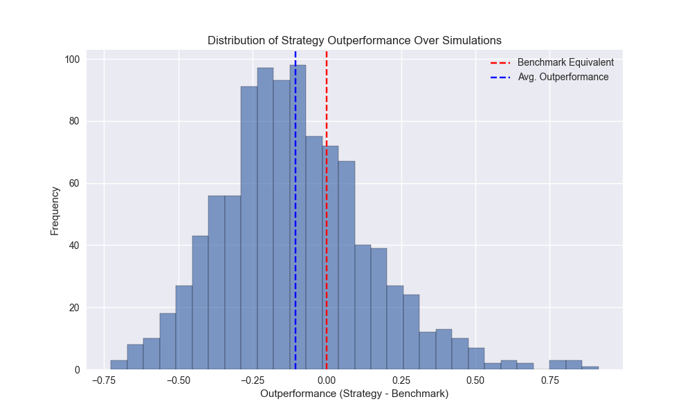
When we run the simulations we find that the strategy has an average underperformance of 11% points vs. buy-and-hold (only slightly better than the 200-day, which was an underperformance of about 13% points). The 12-by-12 returned about 12% on average compared with 9.7% for the 200-day. The Sharpe Ratio is about 0.20 on average, which is less than buy-and-hold of 0.29, but better than the 200-day of 0.15. We show the histogram of the amount of outperformance of the 12-by-12 relative to buy-and-hold below.

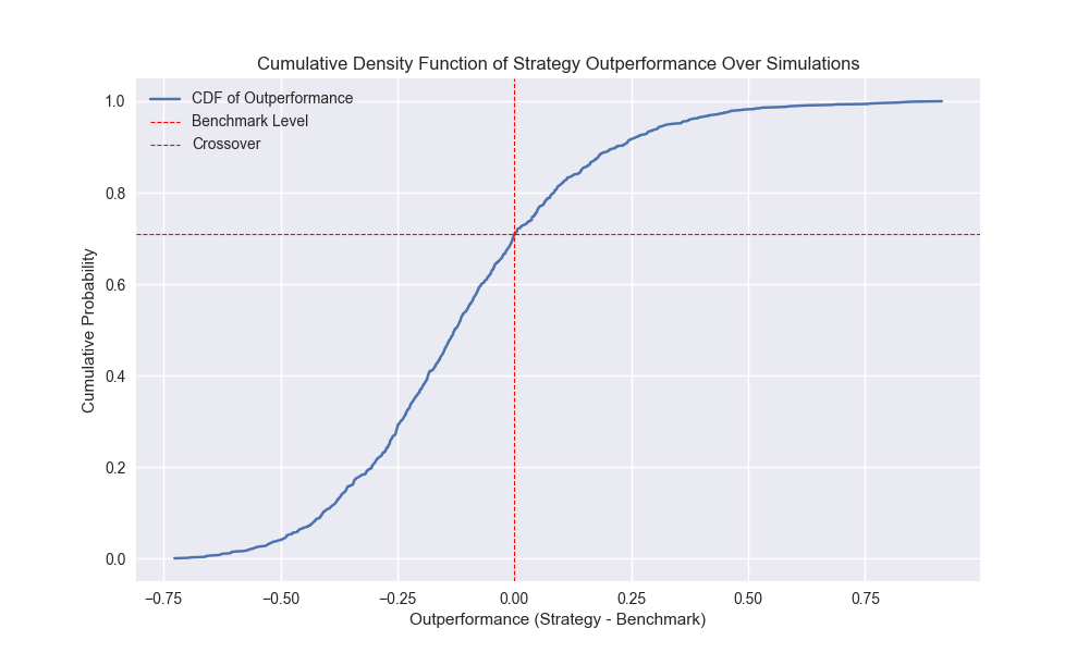
The empirical cumulative distribution function plot shows that the strategy’s cumulative return exceeds buy-and-hold about 29% of the time – not much different than the 200-day – as shown below. The Sharpe ratio outperforms buy-and-hold about 36% of time, better than the 200-day.

Running the simulations with the 7-block sample yields the following summary statistics below.

7-block sample	12-by-12	200-day	Buy-and-Hold
Return	15.6%	9.8%	24.4%
Sharpe Ratio	0.25	0.16	0.31
Return Outperformance Frequency	31.7%	24.8%
Sharpe Outperformance Frequency	38.5%	30.1%

As shown above, the 12-by-12 strategy underperforms buy-and-hold across the simulations. It’s frequency of outperformance is slightly higher at almost 32% than than the 3-block at 28%. Frequency of Sharpe Ratio outperformance is also about 300bps better than the 3-block simulation at close to 39%. Notably, the 7-block sees the 12-by-12 outperform the 200-day in terms of frequency of outperformance relative to buy-and-hold. Unfortunately, this isn’t sufficient to conclude the 12-by-12 is a dramatically better strategy.

So the real question now is, given all the information we’ve compiled so far, should we favor the 12-by-12 strategy? The evidence suggests that while the strategy outperformed buy-and-hold and the 200-day historically, the likelihood it will do so in the future is less than 50/50. Now that we’re two-thirds of the way through our 30 days of backtesting what should we do? File this strategy away with so many others never again to see the light of day? Or investigate ways to improve the strategy if possible? We’ll save that discussion for our next post.

Code below.

# Built using Python 3.10.19 and a virtual environment 

# Load libraries
import pandas as pd
import numpy as np
import yfinance as yf
from datetime import datetime, timedelta
import statsmodels.api as sm
import matplotlib.pyplot as plt
from matplotlib.ticker import FuncFormatter
from utils_intraday import *
from statsmodels.graphics.tsaplots import plot_acf
from statsmodels.tsa.stattools import acf
from tqdm import tqdm

plt.style.use('seaborn-v0_8')
plt.rcParams['figure.figsize'] = (14,8)

def get_spy_weekly_data() -> pd.DataFrame:
    df = yf.download('SPY', start='2000-01-01', end='2024-10-01')
    df.columns = ['open', 'high', 'low', 'close', 'adj close', 'volume']
    df.index.name = 'date'

    # Create training set and downsample to weekly ending Friday
    df_train = df.loc[:'2019-01-01', 'adj close'].copy()
    df_w = pd.DataFrame(df_train.resample('W-FRI').last())
    df_w.columns = ['price'] 

    return df_w

df_w = get_spy_weekly_data()

# Create momentum dictionary
periods = [3, 6, 9, 12]
momo_dict = {}
for back in periods:
    for forward in periods:
        df_out = df_w.copy()
        df_out['ret_back'] = np.log(df_out['price']/df_out['price'].shift(back))
        df_out['ret_for'] = np.log(df_out['price'].shift(-forward)/df_out['price'])
        df_out = df_out.dropna()

        mod = sm.OLS(df_out['ret_for'], sm.add_constant(df_out['ret_back'])).fit()
        momo_dict[f"{back} - {forward}"] = {'data': df_out,
                                            'params': mod.params,
                                            'pvalues': mod.pvalues}

# Prepare model
model_name = '12 - 12'
mod_look_forward = 12
train_pd = 5
test_pd = 1
tot_pd = train_pd + test_pd

df_trade = momo_dict[model_name]['data'].copy()

trade_pred = []
for i in range(tot_pd, len(df_trade)+1, test_pd):
    train_df = df_trade.iloc[i-tot_pd:i-test_pd, 1:]
    test_df = df_trade.iloc[i-test_pd+mod_look_forward-1:i-test_pd+mod_look_forward, 1:]

    # Ensure 'ret_back' is 2D by selecting it as a DataFrame, not a Series
    X_train = sm.add_constant(train_df[['ret_back']])
    if test_df.shape[0] > 1:
        X_test = sm.add_constant(test_df[['ret_back']])
    else:
        X_test = sm.add_constant(test_df[['ret_back']], has_constant='add')

    # Fit the model
    mod_run = sm.OLS(train_df['ret_for'], X_train).fit()

    # Predict using the test data
    mod_pred = mod_run.predict(X_test).values
    trade_pred.extend(mod_pred)

df_trade['pred'] = np.concatenate((np.zeros(mod_look_forward + train_pd - 1), np.array(trade_pred)))
df_trade['ret'] = np.log(df_trade['price']/df_trade['price'].shift(1))

df_trade['signal'] = np.where(df_trade['pred'] > 0, 1, 0)
df_trade['signal_sh'] = np.where(df_trade['pred'] >= 0, 1, -1)

df_trade['strat_ret'] = df_trade['signal'].shift(1) * df_trade['ret']
df_trade['strat_ret_sh'] = df_trade['signal_sh'].shift(1) * df_trade['ret']

# Load data
df = pd.read_csv('data/spy_ief_close.csv', parse_dates=['date'], index_col='date')
df_bw =  pd.DataFrame(df.resample('W-FRI').last())
df_bw[['ief_chg', 'spy_chg']] = df_bw[['ief','spy']].apply(lambda x: np.log(x/x.shift(1)))

end_date_bench = df_trade.index[-1].strftime("%Y-%m-%d")
bench_returns = df_bw[['ief_chg', 'spy_chg']].copy()
bench_returns = bench_returns.loc[:end_date_bench]
bench_returns = bench_returns.dropna()

strat_returns_start = bench_returns.index[0].strftime("%Y-%m-%d")
strat_returns = df_trade['strat_ret'].copy()
strat_returns = strat_returns.loc[strat_returns_start:]

weights = [0.4,0.6]
bench_60_40_rebal = calculate_portfolio_performance(weights, bench_returns, rebalance=False, frequency='quarter')
bench_60_40_rebal.index = bench_60_40_rebal.index.tz_localize(None) #type:ignore

df_200 = df_w.copy()
df_200.columns = ['price']
df_200 = df_200.resample('W-FRI').last()
# 40 weeks = 200 days
df_200['sma_200'] = df_200['price'].rolling(40).mean()
df_200['ret'] = np.log(df_200['price']/df_200['price'].shift(1))
df_200['signal'] = np.where(df_200['price'] > df_200['sma_200'], 1, 0)
df_200['strat_ret'] = df_200['signal'].shift(1)*df_200['ret']
df_200_bench = df_200.loc[df_trade['strat_ret'].index[0]:df_trade['strat_ret'].index[-1]]


# Circular block for 12-by-12 strategy

data = df_w.apply(lambda x: np.log(x/x.shift(1))).dropna().copy()
data = data.loc[:'2019-01-01']

#### 3-block ####
block_size = 3
data_idx = len(data) - 1
# data_len = len(data)
data_len = int(52*5 + 24) # five years + 12 weeks on either end
iter = data_len // block_size 
adder = data_len % block_size
block_data = []

np.random.seed(42)
for _ in tqdm(range(1000), desc='Simulation'):
    dat = []
    for _ in range(iter):
        start = np.random.choice(data_idx, 1)[0]
        end = start+block_size
        out = data.iloc[start:end]
        if end > data_idx + 1:
            new_end = end - data_idx - 1
            new_out = data.iloc[:new_end]
            out = pd.concat([out, new_out])
        dat.extend(out.values)
    if adder:
        new_start = np.random.choice(data_idx, 1)[0]
        new_end = new_start+adder
        out_add = data.iloc[new_start:new_end]
        if new_end > data_idx + 1:
            s_end = new_end - data_idx - 1
            s_end = s_end if s_end < adder else adder - 1 
            new_out = data.iloc[:s_end]
            out_add = pd.concat([out_add, new_out])
        dat.extend(out_add.values)
    block_data.append(dat)

len([idx for idx, val in enumerate(block_data) if len(val)>data_len])

back = 12
forward = 12
mod_look_forward = forward
train_pd = 5
test_pd = 1
tot_pd = train_pd + test_pd

lst_sim = []
for dt in tqdm(block_data, desc='Simulations'):
    price_sim = np.exp(np.array(dt)).cumprod()*100
    dataf = pd.DataFrame(np.c_[price_sim, np.array(dt)], columns=['price', 'ret'])

    dataf['ret_back'] = np.log(dataf['price']/dataf['price'].shift(back))
    dataf['ret_for'] = np.log(dataf['price'].shift(-forward)/dataf['price'])
    dataf = dataf.dropna()

    trade_pred = []
    for i in range(tot_pd, len(dataf)+1, test_pd):
        train_df = dataf.iloc[i-tot_pd:i-test_pd, 2:]
        test_df = dataf.iloc[i-test_pd+mod_look_forward-1:i-test_pd+mod_look_forward, 2:]

        # Ensure 'ret_back' is 2D by selecting it as a DataFrame, not a Series
        X_train = sm.add_constant(train_df[['ret_back']], has_constant='add')
        if test_df.shape[0] > 1:
            X_test = sm.add_constant(test_df[['ret_back']])
        else:
            X_test = sm.add_constant(test_df[['ret_back']], has_constant='add')

        # Fit the model
        mod_run = sm.OLS(train_df['ret_for'], X_train).fit()

        # Predict using the test data
        mod_pred = mod_run.predict(X_test).values
        trade_pred.extend(mod_pred)

    dataf['pred'] = np.concatenate((np.zeros(mod_look_forward + train_pd - 1), np.array(trade_pred)))
    
    dataf['signal'] = np.where(dataf['pred'] > 0, 1, 0)
    dataf['signal_sh'] = np.where(dataf['pred'] >= 0, 1, -1)

    dataf['strat_ret'] = dataf['signal'].shift(1) * dataf['ret']
    dataf['strat_ret_sh'] = dataf['signal_sh'].shift(1) * dataf['ret']

    cumul_ret = dataf[['strat_ret', 'strat_ret_sh', 'ret']].cumsum().iloc[-1].values
    sharpe = dataf[['strat_ret', 'strat_ret_sh', 'ret']].apply(lambda x: x.mean()/x.std()*np.sqrt(52)).values
    lst_sim.append([cumul_ret, sharpe])


flat_data = [np.concatenate(triple) for triple in lst_sim]
df_sim = pd.DataFrame(flat_data, columns=['strat_ret', 'strat_ret_sh', 'ret', 'strat_sharpe','strat_sharpe_sh', 'ret_sharpe'])
df_sim['outperf'] = df_sim['strat_ret'] - df_sim['ret']
df_sim['outperf_sh'] = df_sim['strat_ret_sh'] - df_sim['ret']


# Plot the histogram of outperformance
plt.figure()
plt.hist(df_sim['outperf'], bins=30, alpha=0.7, edgecolor='black')
plt.axvline(0, color='red', linestyle='--', label='Benchmark Equivalent')
plt.axvline(df_sim['outperf'].mean(), color='blue', linestyle='--', label='Avg. Outperformance')
plt.xlabel('Outperformance (Strategy - Benchmark)')
plt.ylabel('Frequency')
plt.title('Distribution of Strategy Outperformance Over Simulations')
plt.legend()
plt.show()

# Plot cumulative distribution function
# Sort the outperformance values
sorted_outperf = np.sort(df_sim['outperf'])

# Calculate cumulative probabilities
cumul_prob = np.arange(1, len(sorted_outperf) + 1) / len(sorted_outperf)
crossover = cumul_prob[(sorted_outperf > -0.001) & (sorted_outperf < 0.001)].mean().round(2)

# Plot the CDF
plt.figure(figsize=(10, 6))
plt.plot(sorted_outperf, cumul_prob, label='CDF of Outperformance')
plt.axvline(0, color='red', linestyle='--', linewidth=0.8, label='Benchmark Level')
plt.axhline(crossover, color='red', linestyle='--', linewidth=0.8, label='Crossover')
plt.xlabel('Outperformance (Strategy - Benchmark)')
plt.ylabel('Cumulative Probability')
plt.title('Cumulative Density Function of Strategy Outperformance Over Simulations')
plt.legend()
plt.show()