Day 21: Drawing Board

On Day 20 we completed our analysis of the 12-by-12 strategy using circular block sampling on the 3 and 7 blocks. We found the strategy did not outperform buy-and-hold on average and its frequency of outperformance was modest – in the 28-31% range – insufficient to warrant actually executing the strategy. What to do? Back to the drawing board to test a new strategy? Or to the water board to torture the current one?

Even though we engaged in a transparent and methodical approach to developing and testing an investment strategy, one could still find flaws in the logic. Is a 12-week look forward target variable all that meaningful for trading? Why should we expect a univariate linear regression to have much predictive power in the first place? Why weren’t we using AR, ARIMA, GAM, VECM, GARCH, or XGGLS¹ models? And why the heck did we conduct this on a weekly basis anyway?

All valid responses and criticisms. One of the main reasons we chose what we chose is to provide analysis that is reproducible, rigorous, and accessible. We also wanted to do it in a narrative fashion so that someone could follow all the steps without undue frustration as to why we made a choice to do something at one step and not another. We want the reading experience to be as enjoyable as possible.² If you don’t feel that to be the case, by all means reach out to content at optionstocksmachines dot com.

Now back to the debate. In reality, this probably isn’t the greatest strategy. But that doesn’t mean we should give up just yet; nor should we knot the model into a pretzel to get a result that looks great for a blog post. Indeed, we have information that should already prove useful. That is, we have a model whose error can be quantified and adjusted. Recall, we had to wait 12 weeks to get the last piece of forward returns to train our model. We then used that model to forecast the next 12 weeks in the most recently completed week. But what if we wait another week to see how the model performs on the next week’s data and then use that error to adjust the forecast using that week’s data?

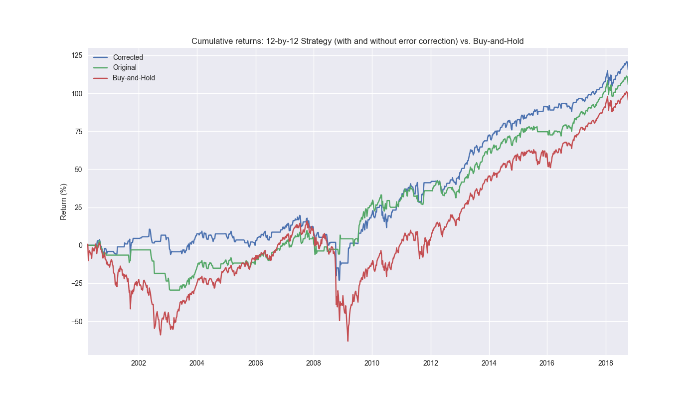
We do just that and show the results in the graph below. The blue line is the strategy with model error correction. The green is the original 12-by-12 strategy without correction. The red line is buy-and-hold. One can see how nicely the error correction improves performance. We’ll discuss this performance and what we did in our next post.

Code below.

# Built using Python 3.10.19 and a virtual environment 

# Load packages
import pandas as pd
import numpy as np
from datetime import datetime, timedelta
import statsmodels.api as sm
import matplotlib.pyplot as plt
from matplotlib.ticker import FuncFormatter
import yfinance as yf

plt.style.use('seaborn-v0_8')
plt.rcParams['figure.figsize'] = (14,8)

def get_spy_weekly_data() -> pd.DataFrame:
    df = yf.download('SPY', start='2000-01-01', end='2024-10-01')
    df.columns = ['open', 'high', 'low', 'close', 'adj close', 'volume']
    df.index.name = 'date'

    # Create training set and downsample to weekly ending Friday
    df_train = df.loc[:'2019-01-01', 'adj close'].copy()
    df_w = pd.DataFrame(df_train.resample('W-FRI').last())
    df_w.columns = ['price'] 

    return df_w

df_w = get_spy_weekly_data()

# Create momentum dictionary
periods = [3, 6, 9, 12]
momo_dict = {}
for back in periods:
    for forward in periods:
        df_out = df_w.copy()
        df_out['ret_back'] = np.log(df_out['price']/df_out['price'].shift(back))
        df_out['ret_for'] = np.log(df_out['price'].shift(-forward)/df_out['price'])
        df_out = df_out.dropna()

        mod = sm.OLS(df_out['ret_for'], sm.add_constant(df_out['ret_back'])).fit()
        momo_dict[f"{back} - {forward}"] = {'data': df_out,
                                            'params': mod.params,
                                            'pvalues': mod.pvalues}

df_trade = momo_dict['12 - 12']['data'].copy()

# Trade with error handling
df_trade_1 = momo_dict['12 - 12']['data'].copy()

mod_look_forward = 12
train_pd = 5
test_pd = 1
tot_pd = train_pd + test_pd
lr = 2

trade_pred = []
trade_pred_un = []
trade_pred_old = []
for i in range(tot_pd, len(df_trade_1)-mod_look_forward+1, test_pd):
    train_df = df_trade_1.iloc[i-tot_pd:i-test_pd, 1:]
    valid_df = df_trade_1.iloc[i-test_pd:i, 1:]
    uncorr_df = df_trade_1.iloc[i-test_pd+mod_look_forward-1:i-test_pd+mod_look_forward, 1:]
    test_df = df_trade_1.iloc[i-test_pd+mod_look_forward:i-test_pd+mod_look_forward+1, 1:]

    # Ensure 'ret_back' is 2D by selecting it as a DataFrame, not a Series
    X_train = sm.add_constant(train_df[['ret_back']])
    if valid_df.shape[0] > 1:
        X_valid = sm.add_constant(valid_df[['ret_back']])
    else:
        X_valid = sm.add_constant(valid_df[['ret_back']], has_constant='add')

    if uncorr_df.shape[0] > 1:
        X_uncorr = sm.add_constant(uncorr_df[['ret_back']])
    else:
        X_uncorr = sm.add_constant(uncorr_df[['ret_back']], has_constant='add')

    if test_df.shape[0] > 1:
        X_test = sm.add_constant(test_df[['ret_back']])
    else:
        X_test = sm.add_constant(test_df[['ret_back']], has_constant='add')

    # Fit the model
    mod = sm.OLS(train_df['ret_for'], X_train).fit()

    # Predict using the test data
    pred = mod.predict(X_valid).values
    actual = valid_df['ret_for'].values
    gamma = -(actual - pred)*lr
    pred_old = mod.predict(X_uncorr)
    trade_pred_old.extend(pred_old)

    mod_pred = mod.predict(X_test).values
    trade_pred_un.extend(mod_pred)
    trade_pred.extend(mod_pred + gamma)

assert len(trade_pred) + mod_look_forward + train_pd == len(df_trade_1)
assert len(trade_pred_un) + mod_look_forward + train_pd == len(df_trade_1)

df_trade_1['pred'] = np.concatenate((np.zeros(mod_look_forward + train_pd), np.array(trade_pred)))
df_trade_1['pred_un'] = np.concatenate((np.zeros(mod_look_forward + train_pd), np.array(trade_pred_un)))
df_trade_1['pred_old'] = np.concatenate((np.zeros(mod_look_forward + train_pd - 1), np.array(trade_pred_old), np.zeros(1)))
df_trade_1['ret'] = np.log(df_trade_1['price']/df_trade_1['price'].shift(1))

df_trade_1['signal'] = np.where(df_trade_1['pred'] > 0, 1, 0)
df_trade_1['signal_un'] = np.where(df_trade_1['pred_un'] > 0, 1, 0)
df_trade_1['signal_old'] = np.where(df_trade_1['pred_old'] > 0, 1, 0)
df_trade_1['signal_sh'] = np.where(df_trade_1['pred'] >= 0, 1, -1)

df_trade_1['strat_ret'] = df_trade_1['signal'].shift(1) * df_trade_1['ret']
df_trade_1['strat_ret_un'] = df_trade_1['signal_un'].shift(1) * df_trade_1['ret']
df_trade_1['strat_ret_old'] = df_trade_1['signal_old'].shift(1) * df_trade_1['ret']
df_trade_1['strat_ret_sh'] = df_trade_1['signal_sh'].shift(1) * df_trade_1['ret']

(df_trade_1[['strat_ret', 'strat_ret_old', 'ret']].cumsum()*100).plot()
plt.ylabel("Return (%)")
plt.xlabel("")
plt.legend(['Corrected', 'Original', 'Buy-and-Hold'])
plt.title('Cumulative returns: 12-by-12 Strategy (with and without error correction) vs. Buy-and-Hold')
plt.show()