Day 22: Error Correction

On Day 21, we wrung our hands with frustration over how to proceed. The results of our circular block sampling suggested we shouldn’t expect a whole lot of outperformance in our 12-by-12 model out-of-sample. To deal with this our choices were, back to the drawing board or off to the waterboard to start over or to torture the data until it told us what we wanted. However, we found a third way, in which we could use the information we already had, to make a few minor tweaks to improve the model. We’ll discuss that tweak today. Note: adding an error correction term was inspired by techniques found in traditional machine learning and the speculative learning series in Prognostikon, a blog we highly recommend that features some innovative approaches to quantitative trading. Any errors in this error correction are, of course, ours!

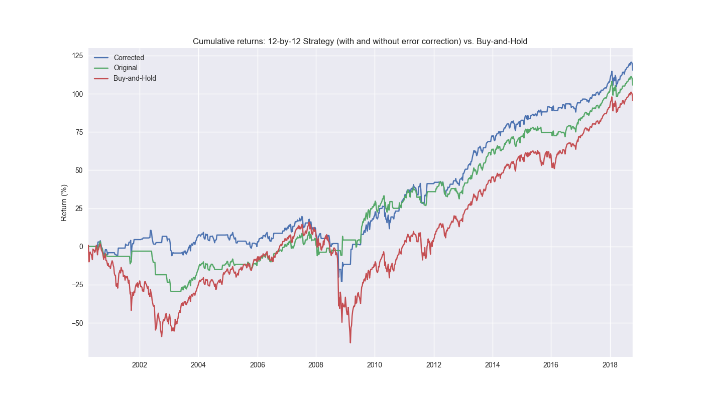
So what did we do? Recall, we had to wait 12 weeks to get the last piece of forward returns to train our model. We then used that model to forecast the next 12 weeks by using the most recently completed week, whose lookback returns went into the last block of the model, as an input to the forecast. That was the 12-by-12 model we’ve been testing. But what we then did was wait another week to see how the model performed on the next week of historical data. We then compared that prediction against the actual and used the error with a little bit of calculus to adjust the forecast. The error term we used is similar to the loss function used in gradient boosting algorithms like XGBoost. (We discuss the loss function in the Appendix after the code.) We add this error to our forecast to adjust the prediction, but keep the same signal generation process. That is, if the prediction is positive go long or hold and if negative close or go short. Let’s look at cumulative performance graphs again. We show the performance of the corrected strategy, the old strategy, and buy-and-hold below.

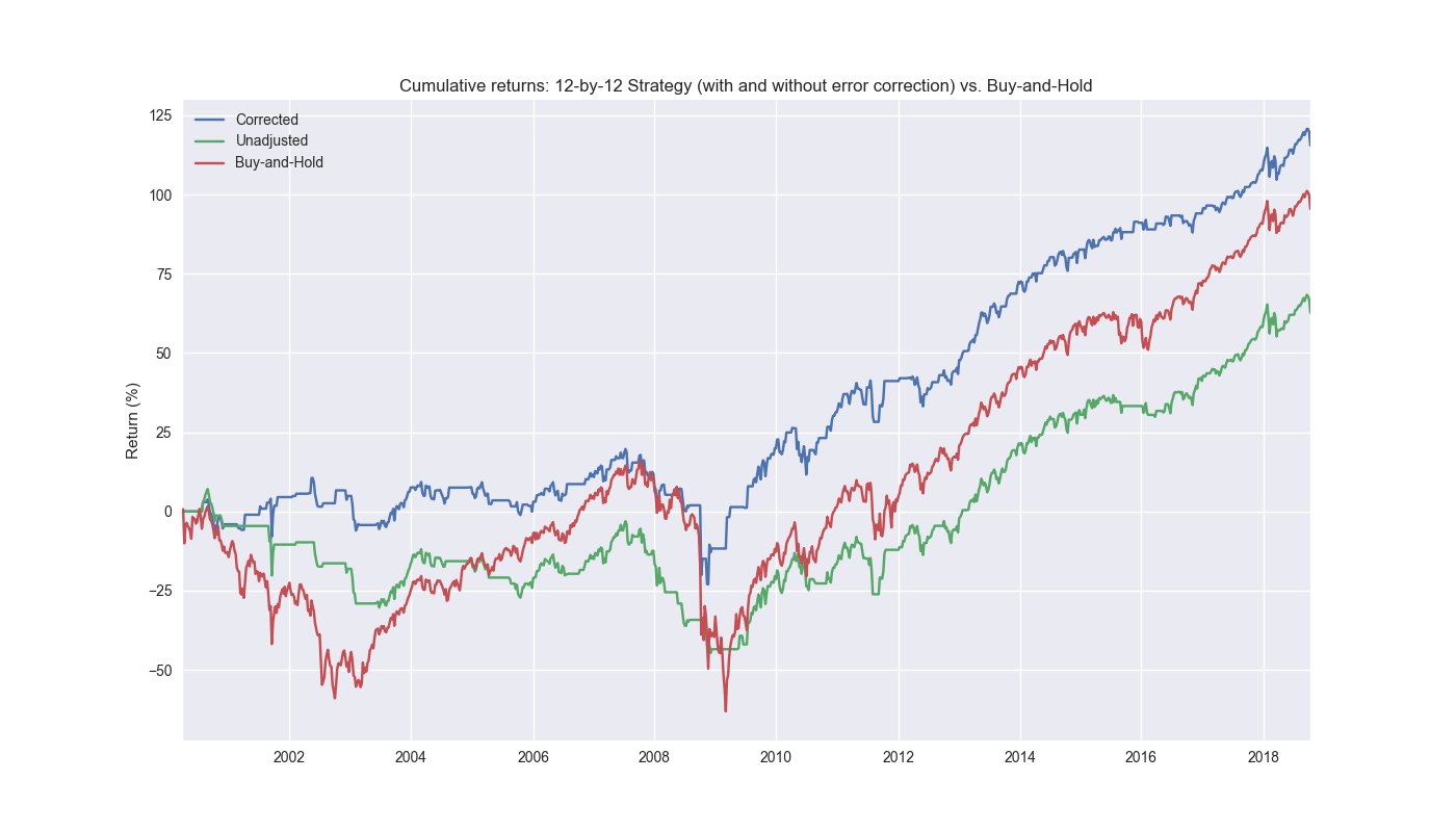
Again, looks pretty nice and definitely warrants further investigation. But before we do that we should look at the corrected strategy, that strategy without the correction, and buy-and-hold.

This is very revealing. The uncorrected strategy actually underperforms all other strategies. What is particularly remarkable, and an open question, is how such a modest modification could turn an underperforming strategy into an outperforming one. Is there a logical basis for it, or is just luck? We’ll consider that in our next post.

Code below.

# Built using Python 3.10.19 and a virtual environment 

# Load packages
import pandas as pd
import numpy as np
from datetime import datetime, timedelta
import statsmodels.api as sm
import matplotlib.pyplot as plt
from matplotlib.ticker import FuncFormatter
import yfinance as yf

plt.style.use('seaborn-v0_8')
plt.rcParams['figure.figsize'] = (14,8)

def get_spy_weekly_data() -> pd.DataFrame:
    df = yf.download('SPY', start='2000-01-01', end='2024-10-01')
    df.columns = ['open', 'high', 'low', 'close', 'adj close', 'volume']
    df.index.name = 'date'

    # Create training set and downsample to weekly ending Friday
    df_train = df.loc[:'2019-01-01', 'adj close'].copy()
    df_w = pd.DataFrame(df_train.resample('W-FRI').last())
    df_w.columns = ['price'] 

    return df_w

df_w = get_spy_weekly_data()

# Create momentum dictionary
periods = [3, 6, 9, 12]
momo_dict = {}
for back in periods:
    for forward in periods:
        df_out = df_w.copy()
        df_out['ret_back'] = np.log(df_out['price']/df_out['price'].shift(back))
        df_out['ret_for'] = np.log(df_out['price'].shift(-forward)/df_out['price'])
        df_out = df_out.dropna()

        mod = sm.OLS(df_out['ret_for'], sm.add_constant(df_out['ret_back'])).fit()
        momo_dict[f"{back} - {forward}"] = {'data': df_out,
                                            'params': mod.params,
                                            'pvalues': mod.pvalues}

df_trade = momo_dict['12 - 12']['data'].copy()

# Trade with error handling
df_trade_1 = momo_dict['12 - 12']['data'].copy()

mod_look_forward = 12
train_pd = 5
test_pd = 1
tot_pd = train_pd + test_pd
lr = 2

trade_pred = []
trade_pred_un = []
trade_pred_old = []
for i in range(tot_pd, len(df_trade_1)-mod_look_forward+1, test_pd):
    train_df = df_trade_1.iloc[i-tot_pd:i-test_pd, 1:]
    valid_df = df_trade_1.iloc[i-test_pd:i, 1:]
    uncorr_df = df_trade_1.iloc[i-test_pd+mod_look_forward-1:i-test_pd+mod_look_forward, 1:]
    test_df = df_trade_1.iloc[i-test_pd+mod_look_forward:i-test_pd+mod_look_forward+1, 1:]

    # Ensure 'ret_back' is 2D by selecting it as a DataFrame, not a Series
    X_train = sm.add_constant(train_df[['ret_back']])
    if valid_df.shape[0] > 1:
        X_valid = sm.add_constant(valid_df[['ret_back']])
    else:
        X_valid = sm.add_constant(valid_df[['ret_back']], has_constant='add')

    if uncorr_df.shape[0] > 1:
        X_uncorr = sm.add_constant(uncorr_df[['ret_back']])
    else:
        X_uncorr = sm.add_constant(uncorr_df[['ret_back']], has_constant='add')

    if test_df.shape[0] > 1:
        X_test = sm.add_constant(test_df[['ret_back']])
    else:
        X_test = sm.add_constant(test_df[['ret_back']], has_constant='add')

    # Fit the model
    mod = sm.OLS(train_df['ret_for'], X_train).fit()

    # Predict using the test data
    pred = mod.predict(X_valid).values
    actual = valid_df['ret_for'].values
    gamma = -(actual - pred)*lr
    pred_old = mod.predict(X_uncorr)
    trade_pred_old.extend(pred_old)

    mod_pred = mod.predict(X_test).values
    trade_pred_un.extend(mod_pred)
    trade_pred.extend(mod_pred + gamma)

assert len(trade_pred) + mod_look_forward + train_pd == len(df_trade_1)
assert len(trade_pred_un) + mod_look_forward + train_pd == len(df_trade_1)

df_trade_1['pred'] = np.concatenate((np.zeros(mod_look_forward + train_pd), np.array(trade_pred)))
df_trade_1['pred_un'] = np.concatenate((np.zeros(mod_look_forward + train_pd), np.array(trade_pred_un)))
df_trade_1['pred_old'] = np.concatenate((np.zeros(mod_look_forward + train_pd - 1), np.array(trade_pred_old), np.zeros(1)))
df_trade_1['ret'] = np.log(df_trade_1['price']/df_trade_1['price'].shift(1))

df_trade_1['signal'] = np.where(df_trade_1['pred'] > 0, 1, 0)
df_trade_1['signal_un'] = np.where(df_trade_1['pred_un'] > 0, 1, 0)
df_trade_1['signal_old'] = np.where(df_trade_1['pred_old'] > 0, 1, 0)
df_trade_1['signal_sh'] = np.where(df_trade_1['pred'] >= 0, 1, -1)

df_trade_1['strat_ret'] = df_trade_1['signal'].shift(1) * df_trade_1['ret']
df_trade_1['strat_ret_un'] = df_trade_1['signal_un'].shift(1) * df_trade_1['ret']
df_trade_1['strat_ret_old'] = df_trade_1['signal_old'].shift(1) * df_trade_1['ret']
df_trade_1['strat_ret_sh'] = df_trade_1['signal_sh'].shift(1) * df_trade_1['ret']

(df_trade_1[['strat_ret', 'strat_ret_old', 'ret']].cumsum()*100).plot()
plt.ylabel("Return (%)")
plt.xlabel("")
plt.legend(['Corrected', 'Original', 'Buy-and-Hold'])
plt.title('Cumulative returns: 12-by-12 Strategy (with and without error correction) vs. Buy-and-Hold')
plt.show()