Day 25: Positives and Negatives

On Day 24, we explained in detail how the error correction term led to somewhat unexpected outperformance relative to the original and unadjusted strategies. The reason? We hypothesized that it was due to the the error term adjusting the prediction in a trending direction when or if the current walk-forward model was mean reverting. We noted that the walk-forward models tended to have negative size effects, so were likely mean reverting. Hence, while each model might tend to predict some sort of reversion once a baseline threshold was surpassed, if the near-term direction was still trending, adding the error correction might override that forecast and keep the trade going.

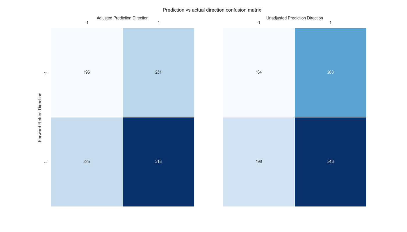
Clearly, the error correction won’t be successful all the time. But, as we showed in our last post, it does tend to predict the near-term downside better than the unadjusted model. Here’s the confusion matrix again.

Now how should we judge these results? Two errors really matter when predicting direction. Incorrectly predicting a positive return when it is in fact negative. And incorrectly predicting a negative return when it is in fact positive. In other words, false positives and false negatives.¹ In the case of the adjusted and unadjusted strategies above, we can see that the adjusted strategy has far fewer false positives at 231 than the unadjusted at 263. However, the adjusted strategy has decidedly more false negatives than the unadjusted at 225 vs. 198. Of course, the adjusted strategy’s true positives fall short of the unadjusted’s at 316 vs. 343. But its true negatives exceed the unadjusted’s meaningfully at 196 vs. 164.

As we joked, the first rule of trading is don’t lose money. And that seems borne out by these results. Even though the unadjusted strategy nails the upside more often, that the adjusted strategy picks the downside better, seems to win the day. But if we should also be concerned with false positives and false negatives, which is worse? In some sense, it depends on the market. In upward trending markets, false negatives hurt more. In bear markets, false positives. In one you miss the upside, in the other you suffer the downside.

One would think that across a cycle false positives might be the one to avoid over false negatives. The main reason: markets don’t crash up, as the old saw goes. Negative returns are frequently larger in absolute terms than positive ones. On the other hand, there are often a few sizeable up days that make one’s year. Indeed, the internet is chock full of articles on The Ten Best Days of… pick your market. These articles are usually meant to prove that you should always stay fully invested because you can’t time the market. Never mind that such articles are often written by well-intentioned advisors whose fee structure is based on percent of assets under management. Whatever. Let’s move on.

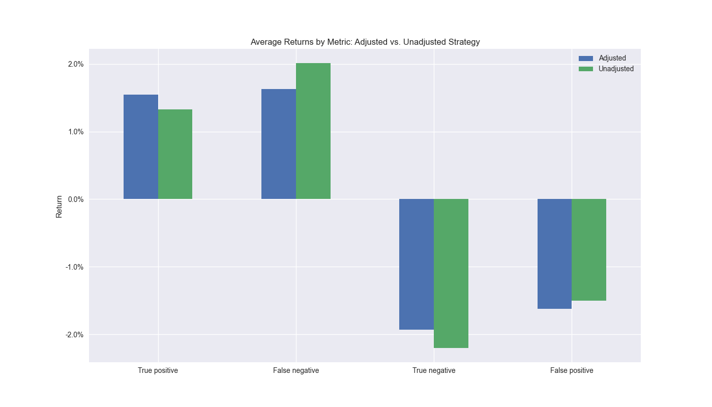
We want to calculate how much the error costs the trading strategy as well as how much the correct signal benefits it. We do so in the graph below.

As one can see based on the true positives, the adjusted strategy has a higher average return than the unadjusted despite having fewer instances of correct forecasts. The adjusted strategy also has a lower average return than the unadjusted for false negatives, meaning that when it incorrectly predicts a down market, the strategy doesn’t suffer as much. On the true negative side, the unadjusted strategy performs better. This might seem counter-intuitive since the unadjusted strategy’s returns are lower than the adjusted. But recall, these are the returns we want the strategy to avoid, so this is the desired performance.² Finally, the adjusted strategy suffers a worse false positive average return than the unadjusted strategy.

While some of the differences we’ve highlighted might not be statistically significant, this has been a lot to digest, so we’ll save the remainder of the discussion for our next post. Code below!

# Built using Python 3.10.19 and a virtual environment 

# Load packages
import pandas as pd
import numpy as np
from datetime import datetime, timedelta
import statsmodels.api as sm
import matplotlib.pyplot as plt
from matplotlib.ticker import FuncFormatter
import yfinance as yf
import seaborn as sns

plt.style.use('seaborn-v0_8')
plt.rcParams['figure.figsize'] = (14,8)

def get_spy_weekly_data() -> pd.DataFrame:
    df = yf.download('SPY', start='2000-01-01', end='2024-10-01')
    df.columns = ['open', 'high', 'low', 'close', 'adj close', 'volume']
    df.index.name = 'date'

    # Create training set and downsample to weekly ending Friday
    df_train = df.loc[:'2019-01-01', 'adj close'].copy()
    df_w = pd.DataFrame(df_train.resample('W-FRI').last())
    df_w.columns = ['price'] 

    return df_w

df_w = get_spy_weekly_data()

# Create momentum dictionary
periods = [3, 6, 9, 12]
momo_dict = {}
for back in periods:
    for forward in periods:
        df_out = df_w.copy()
        df_out['ret_back'] = np.log(df_out['price']/df_out['price'].shift(back))
        df_out['ret_for'] = np.log(df_out['price'].shift(-forward)/df_out['price'])
        df_out = df_out.dropna()

        mod = sm.OLS(df_out['ret_for'], sm.add_constant(df_out['ret_back'])).fit()
        momo_dict[f"{back} - {forward}"] = {'data': df_out,
                                            'params': mod.params,
                                            'pvalues': mod.pvalues}

# df_trade = momo_dict['12 - 12']['data'].copy()

# Trade with error handling
df_trade_1 = momo_dict['12 - 12']['data'].copy()

mod_look_forward = 12
train_pd = 5
test_pd = 1
tot_pd = train_pd + test_pd
lr = 2

trade_pred = []
trade_pred_un = []
trade_pred_old = []
for i in range(tot_pd, len(df_trade_1)-mod_look_forward+1, test_pd):
    train_df = df_trade_1.iloc[i-tot_pd:i-test_pd, 1:]
    valid_df = df_trade_1.iloc[i-test_pd:i, 1:]
    uncorr_df = df_trade_1.iloc[i-test_pd+mod_look_forward-1:i-test_pd+mod_look_forward, 1:]
    test_df = df_trade_1.iloc[i-test_pd+mod_look_forward:i-test_pd+mod_look_forward+1, 1:]

    # Ensure 'ret_back' is 2D by selecting it as a DataFrame, not a Series
    X_train = sm.add_constant(train_df[['ret_back']])
    if valid_df.shape[0] > 1:
        X_valid = sm.add_constant(valid_df[['ret_back']])
    else:
        X_valid = sm.add_constant(valid_df[['ret_back']], has_constant='add')

    if uncorr_df.shape[0] > 1:
        X_uncorr = sm.add_constant(uncorr_df[['ret_back']])
    else:
        X_uncorr = sm.add_constant(uncorr_df[['ret_back']], has_constant='add')

    if test_df.shape[0] > 1:
        X_test = sm.add_constant(test_df[['ret_back']])
    else:
        X_test = sm.add_constant(test_df[['ret_back']], has_constant='add')

    # Fit the model
    mod = sm.OLS(train_df['ret_for'], X_train).fit()

    # Predict using the test data
    pred = mod.predict(X_valid).values
    actual = valid_df['ret_for'].values
    gamma = -(actual - pred)*lr
    # gamma = -1 if np.sign(actual) + np.sign(pred) == 0 else 1
    pred_old = mod.predict(X_uncorr)
    trade_pred_old.extend(pred_old)

    mod_pred = mod.predict(X_test).values
    trade_pred_un.extend(mod_pred)
    trade_pred.extend(mod_pred + gamma)

assert len(trade_pred) + mod_look_forward + train_pd == len(df_trade_1)
assert len(trade_pred_un) + mod_look_forward + train_pd == len(df_trade_1)

df_trade_1['pred'] = np.concatenate((np.zeros(mod_look_forward + train_pd), np.array(trade_pred)))
df_trade_1['pred_un'] = np.concatenate((np.zeros(mod_look_forward + train_pd), np.array(trade_pred_un)))
df_trade_1['pred_old'] = np.concatenate((np.zeros(mod_look_forward + train_pd - 1), np.array(trade_pred_old), np.zeros(1)))
df_trade_1['ret'] = np.log(df_trade_1['price']/df_trade_1['price'].shift(1))

df_trade_1['signal'] = np.where(df_trade_1['pred'] > 0, 1, 0)
df_trade_1['signal_un'] = np.where(df_trade_1['pred_un'] > 0, 1, 0)
df_trade_1['signal_old'] = np.where(df_trade_1['pred_old'] > 0, 1, 0)
df_trade_1['signal_sh'] = np.where(df_trade_1['pred'] >= 0, 1, -1)

df_trade_1['strat_ret'] = df_trade_1['signal'].shift(1) * df_trade_1['ret']
df_trade_1['strat_ret_un'] = df_trade_1['signal_un'].shift(1) * df_trade_1['ret']
df_trade_1['strat_ret_old'] = df_trade_1['signal_old'].shift(1) * df_trade_1['ret']
df_trade_1['strat_ret_sh'] = df_trade_1['signal_sh'].shift(1) * df_trade_1['ret']

df_trade_1['gamma'] = df_trade_1['pred'].sub(df_trade_1['pred_un'])

# Sign analysis
df_corr = df_trade_1[['pred', 'pred_un', 'pred_old', 'gamma', 'ret', 'ret_for', 'ret_back']].copy()

# Convert values to sign: -1 (negative), 0 (neutral), 1 (positive)
pred_sign = [1 if x == 1 else -1 for x in np.sign(df_corr['pred'])]
pred_un_sign = [1 if x == 1 else -1 for x in np.sign(df_corr['pred_un'])]
ret_sign = [1 if x == 1 else -1 for x in np.sign(df_corr['ret_lag'])]
pred_old_sign = [1 if x == 1 else -1 for x in np.sign(df_corr['pred_old'])]

# Create a DataFrame
pred_data = pd.DataFrame({'Prediction': pred_sign, 'Return': ret_sign})
pred_un_data = pd.DataFrame({'Prediction': pred_un_sign, 'Return': ret_sign})

# Create a heatmap of counts for each combination
pred_heatmap = pred_data.groupby(['Prediction', 'Return']).size().unstack(fill_value=0)

pred_un_heatmap = pred_un_data.groupby(['Prediction', 'Return']).size().unstack(fill_value=0)

# Annotations for confusion matrix
annot1 = pred_heatmap_percent.applymap(lambda x: f"{x:.1f}%").values
annot2 = pred_un_heatmap_percent.applymap(lambda x: f"{x:.1f}%").values
annot3 = pred_old_heatmap_percent.applymap(lambda x: f"{x:.1f}%").values

# Heatmap
fig, (ax1, ax2) = plt.subplots(1,2, sharey=True)
fig.text(0.4, 0.95, "Prediction vs actual direction confusion matrix", fontsize=12)

sns.heatmap(pred_heatmap, annot=True, fmt='d', cmap='Blues', cbar=False, linewidths=0.5, linecolor='white', ax=ax1)
ax1.xaxis.tick_top()
ax1.xaxis.set_label_position('top')  # Move the x-axis label to the top
ax1.set_xlabel('Adjusted Prediction Direction', fontsize = 10)
ax1.set_ylabel('Forward Return Direction')

sns.heatmap(pred_un_heatmap, annot=True, fmt='d', cmap='Blues', cbar=False, linewidths=0.5, linecolor='white', ax=ax2)
ax2.xaxis.tick_top()
ax2.xaxis.set_label_position('top')  # Move the x-axis label to the top
ax2.set_xlabel('Unadjusted Prediction Direction', fontsize = 10)
ax2.set_ylabel('')

plt.show()

# Create function to calculate returns by metric
def get_error_df(dataf, pred_col, comp_col, act_col):
    false_positive = dataf.loc[(dataf[pred_col] > 0) & (dataf[act_col] <= 0), act_col].mean()*100

    false_positive_un = dataf.loc[(dataf[comp_col] > 0) & (dataf[act_col] <= 0), act_col].mean()*100

    false_negative = dataf.loc[(dataf[pred_col] <= 0) & (dataf[act_col] > 0), act_col].mean()*100

    false_negative_un = dataf.loc[(dataf[comp_col] <= 0) & (dataf[act_col] > 0), act_col].mean()*100

    true_positive = dataf.loc[(dataf[pred_col] > 0) & (dataf[act_col] > 0), act_col].mean()*100
    true_positive_un = dataf.loc[(dataf[comp_col] > 0) & (dataf[act_col] > 0), act_col].mean()*100

    true_negative = dataf.loc[(dataf[pred_col] < 0) & (dataf[act_col] < 0), act_col].mean()*100
    true_negative_un = dataf.loc[(dataf[comp_col] < 0) & (dataf[act_col] < 0), act_col].mean()*100

    return pd.DataFrame({'Adjusted': [true_positive, false_negative, true_negative, false_positive],
                'Unadjusted': [true_positive_un, false_negative_un, true_negative_un ,false_positive_un]},
                index=['True positive', 'False negative', 'True negative' ,'False positive']
                )

# Create true and false dataframe
df_error = get_error_df(df_corr, 'pred', 'pred_un', 'ret_lag')

# Plot dataframe
df_error.plot(kind='bar', stacked=False, rot=0)
plt.ylabel("Return")
plt.title('Average Returns by Metric: Adjusted vs. Unadjusted Strategy')
plt.yticks([-2.0, -1.0, 0.0, 1.0, 2.0], [f"{x:0.1f}%" for x in [-2.0, -1.0, 0.0, 1.0, 2.0]])
plt.savefig("images/perf_metrics_adj_v_unadj.png")
plt.show()